Exercise 3: Inverse transform sampling

Program a sampling algorithm to sample from the exponential distribution with parameter $\lambda$ thanks to the inverse transform function (starting from the function runif()).
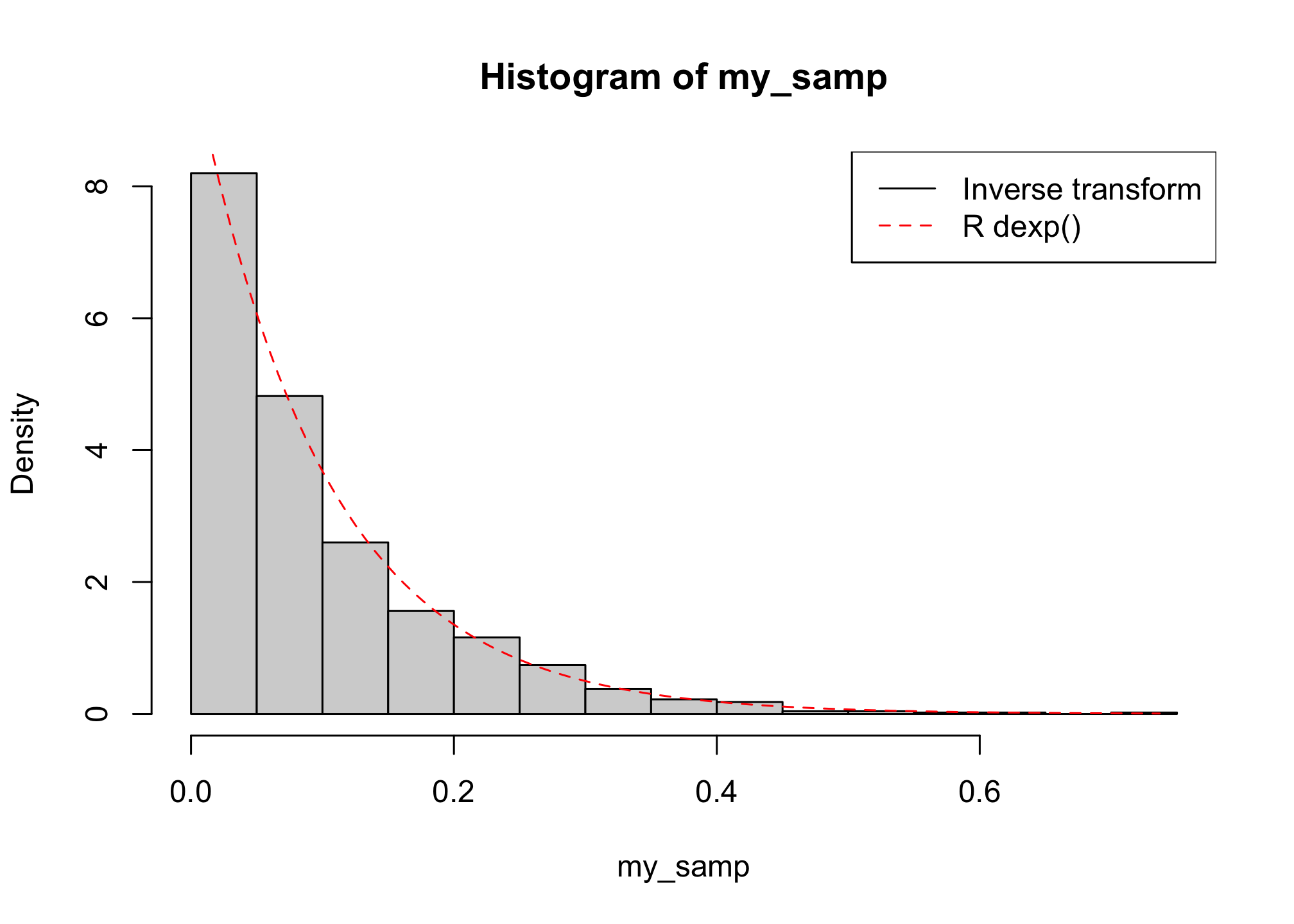
Compare the distribution of your sample to the theoretical target distribution (thanks to the built-in function dexp()).
Try out several values for the $\lambda$ parameter of the exponential distribution (e.g. 1, 10, 0.78, …) to check that the algorithm is indeed working.

generate_exp <- function(n, lambda) {
    u <- runif(n)
    x <- -1/lambda * log(1 - u)
    return(x)
}

n_samp <- 1000
my_samp <- generate_exp(n = n_samp, lambda = 10)
hist(my_samp, probability = TRUE, n = 25)
curve(dexp(x, rate = 10), from = 0, to = max(my_samp), col = "red", lty = 2, add = TRUE)
legend("topright", c("Inverse transform", "R dexp()"), lty = c(1, 2), col = c("black",
    "red"))