Exercise 8: Bayesian regression

We will now analyze data from the therapeutic clinical trial ALBI-ANRS 070 which compared the efficacy and tolerance of 3 anti-retroviral strategies among HIV-1 positive patients naive of any anti-retroviral treatment ¹.

Load the data from the albianrs_data.csv available here (ProTip: set stringsAsFactors = TRUE in read.delim())

  albi <- read.csv("albianrs_data.csv", stringsAsFactors = TRUE)
  summary(albi)

##    PatientID     ViralLoad          CD4              CD4t       CD4sup500
##  ID112  :  7   Min.   :1.699   Min.   : 149.0   Min.   :3.494   No :558  
##  ID130  :  7   1st Qu.:2.042   1st Qu.: 377.0   1st Qu.:4.406   Yes:392  
##  ID139  :  7   Median :2.712   Median : 465.0   Median :4.644            
##  ID15   :  7   Mean   :2.907   Mean   : 491.8   Mean   :4.664            
##  ID156  :  7   3rd Qu.:3.692   3rd Qu.: 585.0   3rd Qu.:4.918            
##  ID163  :  7   Max.   :5.604   Max.   :1318.0   Max.   :6.025            
##  (Other):908                                                             
##    Treatment        Day             Visit      
##  AZT+3TC:315   Min.   :  0.00   Min.   :0.000  
##  d4t+ddI:322   1st Qu.: 29.00   1st Qu.:1.000  
##  switch :313   Median : 84.00   Median :3.000  
##                Mean   : 86.19   Mean   :2.946  
##                3rd Qu.:140.00   3rd Qu.:5.000  
##                Max.   :256.00   Max.   :6.000  
##

The following variables are available:

PatientID : Patient ID
ViralLoad: Plasma viral load
CD4: CD4 T-cell lymphocites rate (in cell/mm³)
CD4t: transformed CD4 T-cell lymphocites rate (in cell/mm³) (CD4t = CD4^1/4)
CD4sup500: binary variable indicating wether CD4 cell counts is above 500
Treatment : Treatment group \(1\) (d4t + ddI), \(2\) (alternance) ou \(3\) (AZT + 3TC))
Day: Day of visit (since inclusion)
Visit: Visit number

Below is a quantitative summary of the characteristics of those variables.

Table 1: **Summary of the Albi-ANRS-070 trial data**
Variable	N = 950¹
ViralLoad	2.71 (2.04, 3.70)
CD4	465 (377, 585)
CD4t	4.64 (4.41, 4.92)
CD4sup500	392 (41%)
Treatment
AZT+3TC	315 (33%)
d4t+ddI	322 (34%)
switch	313 (33%)
Day	84 (29, 140)
Visit
0	146 (15%)
1	140 (15%)
2	136 (14%)
3	130 (14%)
4	128 (13%)
5	135 (14%)
6	135 (14%)
¹ Median (IQR) or n (%)

NB: for simplicity, NA values have been omitted.

First, we want to explain the CD4 rate (as a transformed variable) from the viral load

Display CD4t in scatterplot as a function of the ViralLoad and color the points according to Treatment.

library(ggplot2)
library(MetBrewer)
ggplot(albi, aes(y = CD4t, x = ViralLoad, color = Treatment)) + 
  geom_point(alpha=0.7) +
  MetBrewer::scale_color_met_d("Java") +
  theme_bw()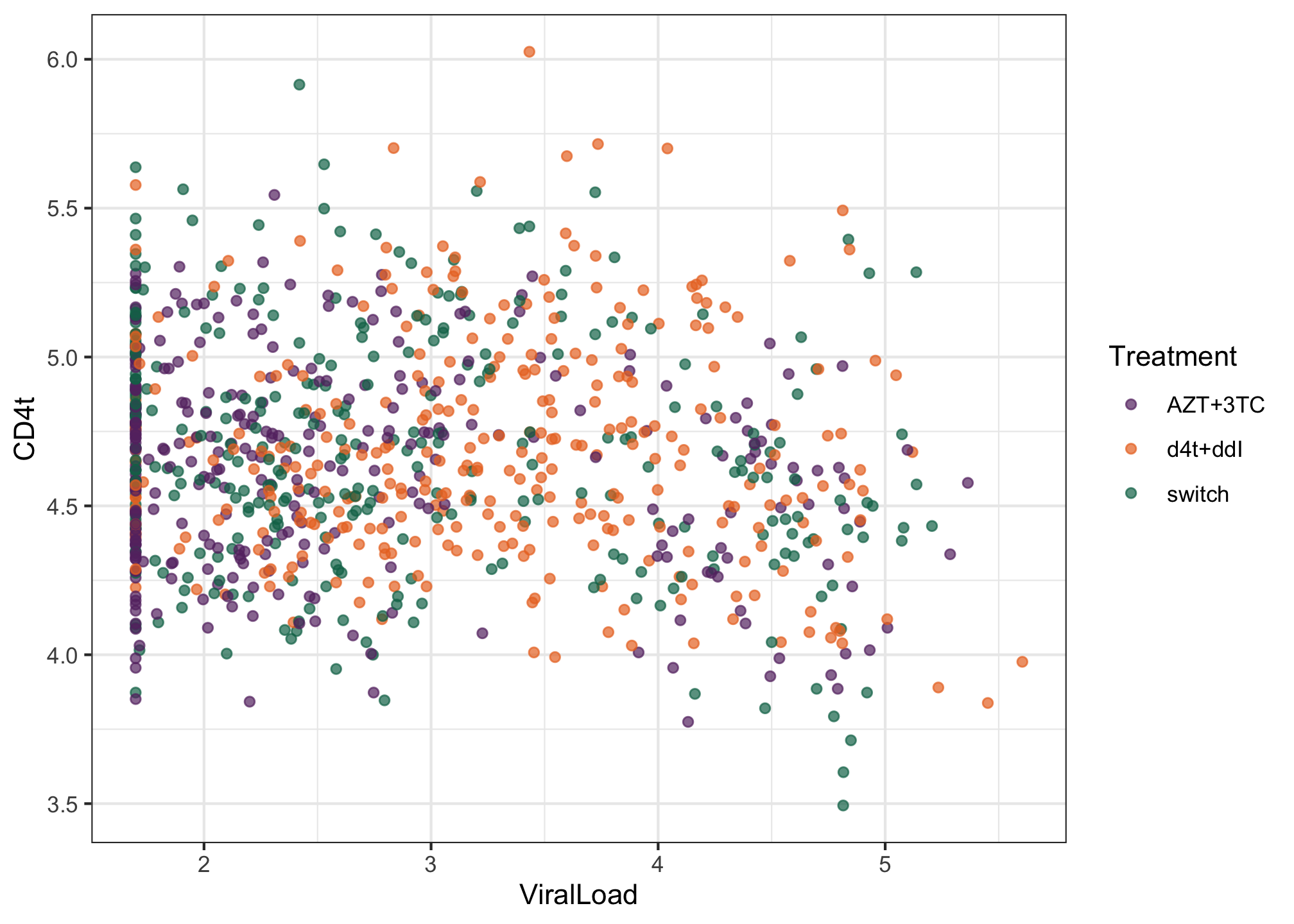

Write down the Bayesian mathematical model corresponding to a linear regression of CD4t against the ViralLoad.

I) Question of interest:
How does the viral load linearly explains the (transformed) CD4 T-cell rate ?
II) Sampling model:
Let \(CD4t_{i}\) be the \(i^{\text{th}}\) (transformed) CD4 T-cell rate \(i\) and \(VL_i^2\) the corresponding observed viral load: \[CD4t_i \overset{iid}{\sim} \mathcal{N}(\beta_0 + \beta_1 VL_i, \sigma^2)\] III) Priors: \[\beta_0\sim \mathcal{N}(0,100^2)\] \[\beta_1 \sim \mathcal{N}(0,100^2)\] \[\sigma^2 \sim InvGamma(0.001,0.001)\]

Write the corresponding BUGS model and save it in an external .txt file.

# Fixed effect linear regression Albi-ANRS
model{

  # Likelihood
  for (i in 1:N){ 
    CD4t[i]~dnorm(mu[i], tau)
    mu[i] <- beta0 + beta1*VL[i]
  }

  # Priors
  beta0~dnorm(0,0.0001) 
  beta1~dnorm(0,0.0001) # proper but very flat (vague: weakly informative)
  tau~dgamma(0.0001,0.0001) # proper but very flat (vague: weakly informative)

  # Parameters of interest
  sigma <- pow(tau, -0.5)
}

Create the corresponding jags object in and generate a Monte Carlo sample of size 1000 for the 3 parameters of interest

library(rjags)
albi_fixed_jags <- jags.model("albiBUGSmodel_fixed.txt", 
                              data = list('CD4t' =  albi$CD4t, 
                                          'N' = nrow(albi), 
                                          'VL' = albi$ViralLoad), 
                              n.chains = 3)

## Compiling model graph
##    Resolving undeclared variables
##    Allocating nodes
## Graph information:
##    Observed stochastic nodes: 950
##    Unobserved stochastic nodes: 3
##    Total graph size: 3195
## 
## Initializing model

res_albi_fixed <- coda.samples(model = albi_fixed_jags, 
                               variable.names = c('beta0', 'beta1', 'sigma'), 
                               n.iter = 1000)

Before interpreting the results, check the convergence. What do you notice ?

  library(coda)
  plot(res_albi_fixed)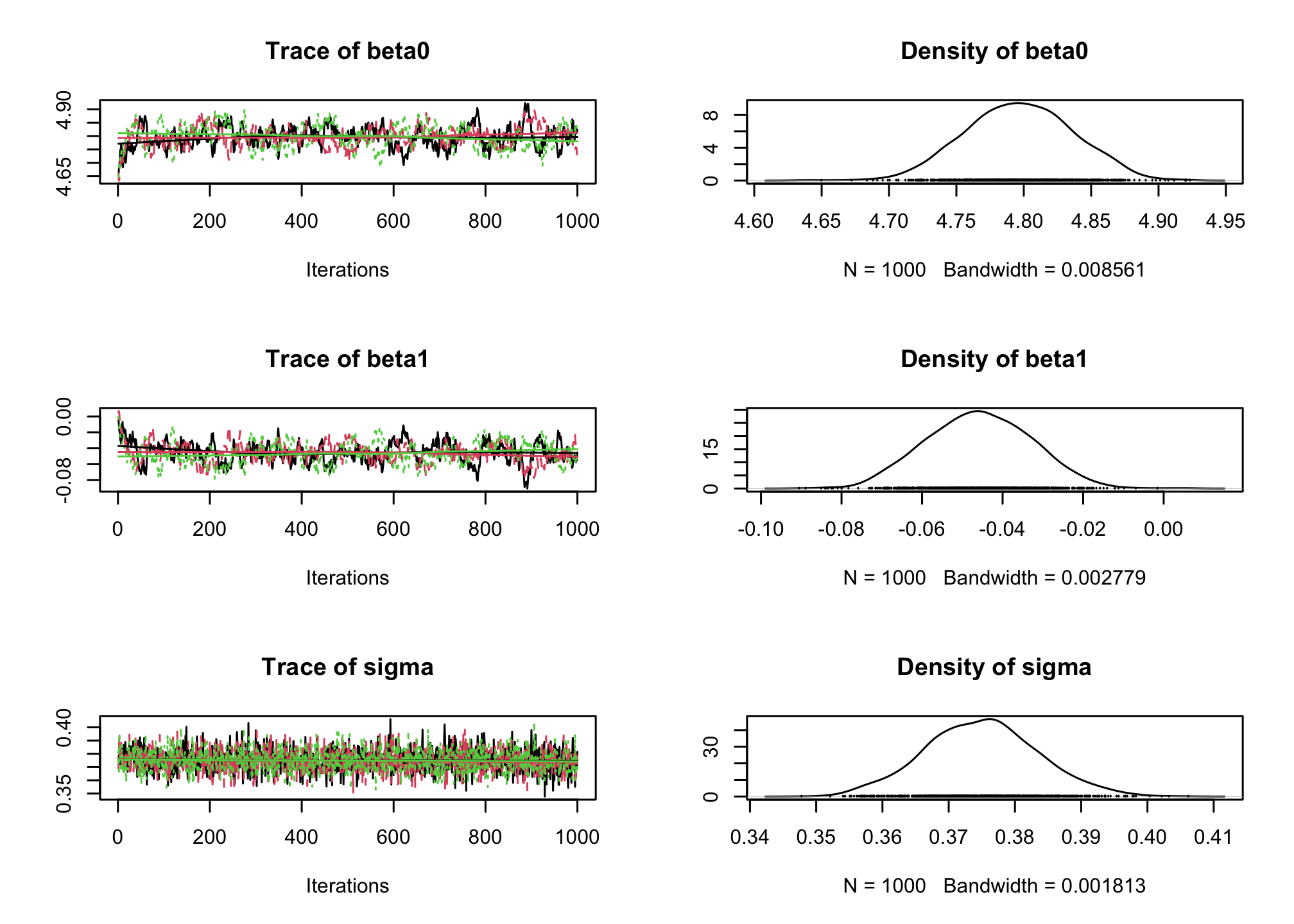

  gelman.plot(res_albi_fixed)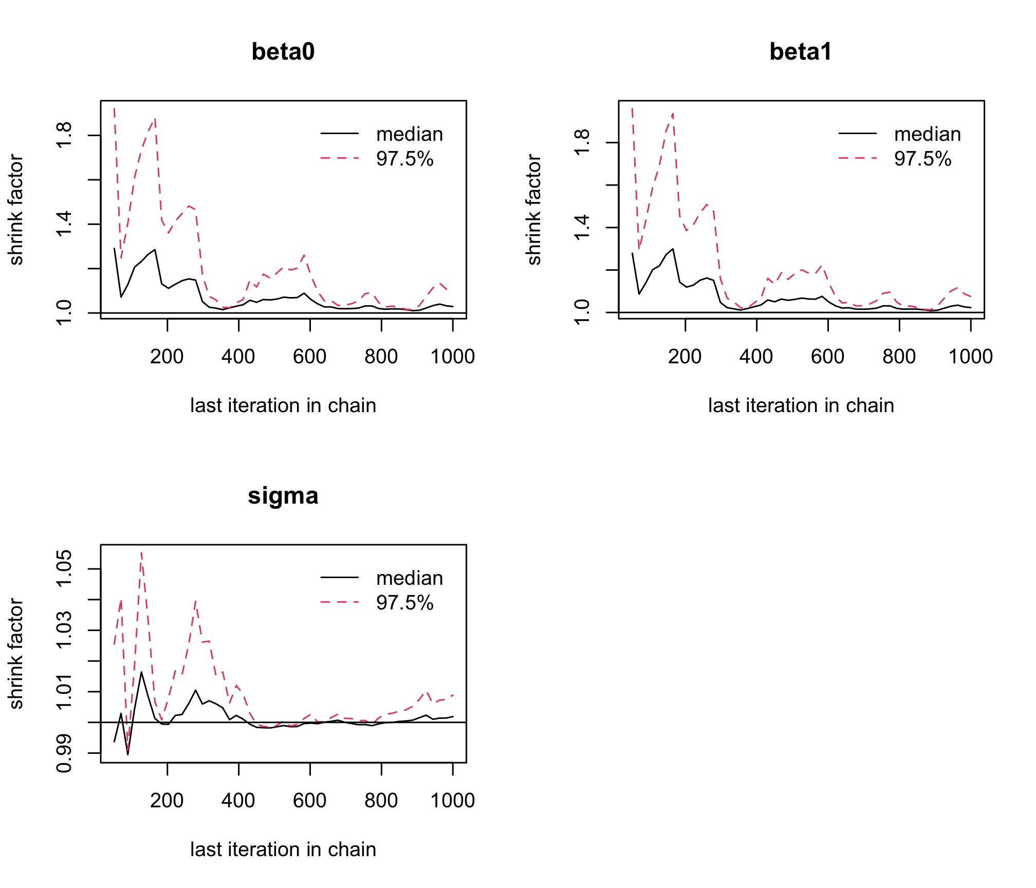

  acfplot(res_albi_fixed)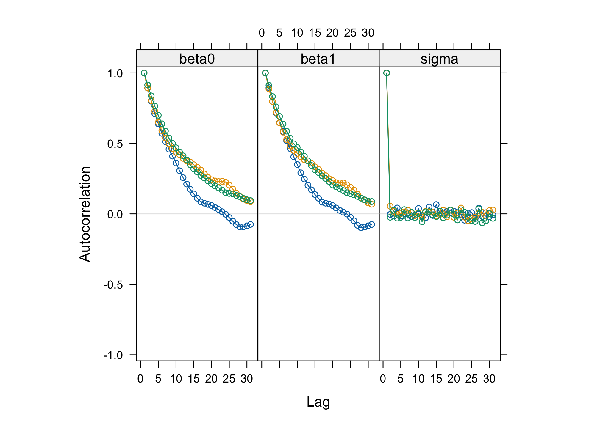

  par(mfrow=c(3, 3))
  cumuplot(res_albi_fixed, ask = FALSE, auto.layout = FALSE)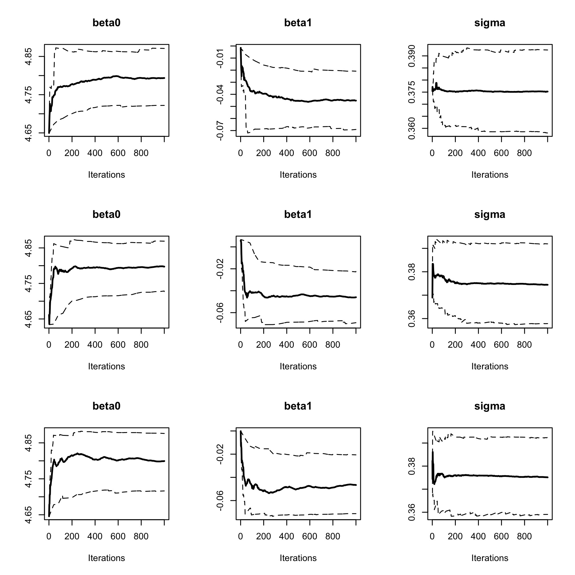

Using the window function, remove the 500 first iterations as burn-in to reach Markov Chain convergence to its stationary distribution (the posterior). Is it sufficient to solve convergence issues ?
```
  res_albi_fixed2 <- window(res_albi_fixed, start=501)

  gelman.plot(res_albi_fixed2)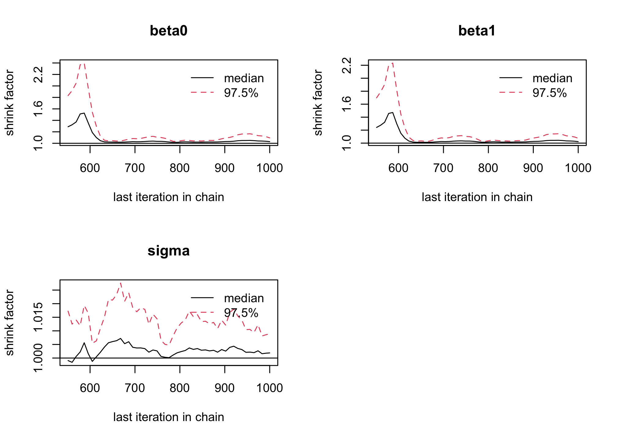
```
```
  acfplot(res_albi_fixed2)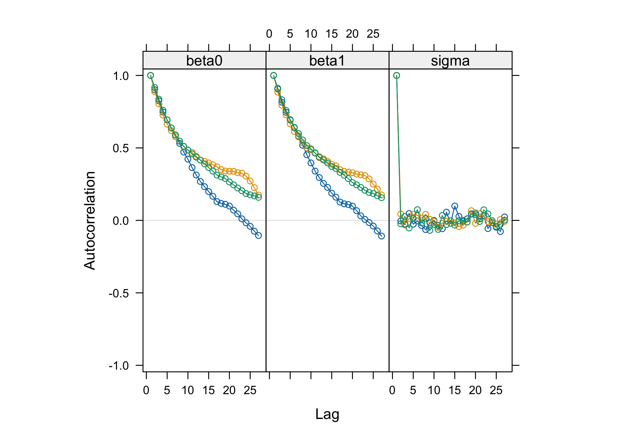
```

Check the effective sample size of the Monte Carlo sample with the effectiveSize() function. Reduuce auto-corrlation by increasing the thin parameter to 10 in coda.samples. Check the impact on the effective sample

?effectiveSize
effectiveSize(res_albi_fixed2)

##      beta0      beta1      sigma 
##   97.64654  104.88987 1703.04910

albi_fixed_jags <- jags.model("albiBUGSmodel_fixed.txt", 
                              data = list('CD4t' =  albi$CD4t, 
                                          'N' = nrow(albi), 
                                          'VL' = albi$ViralLoad), 
                              n.chains = 3)

## Compiling model graph
##    Resolving undeclared variables
##    Allocating nodes
## Graph information:
##    Observed stochastic nodes: 950
##    Unobserved stochastic nodes: 3
##    Total graph size: 3195
## 
## Initializing model

res_albi_fixed_thin <- coda.samples(model = albi_fixed_jags, 
                                    variable.names = c('beta0', 'beta1', 'sigma'), 
                                    n.iter = 10000, thin = 10)
res_albi_fixed_thin <- window(res_albi_fixed_thin, start=5001)

effectiveSize(res_albi_fixed_thin)

##     beta0     beta1     sigma 
##  850.7312  865.1286 1678.9293

plot(res_albi_fixed_thin)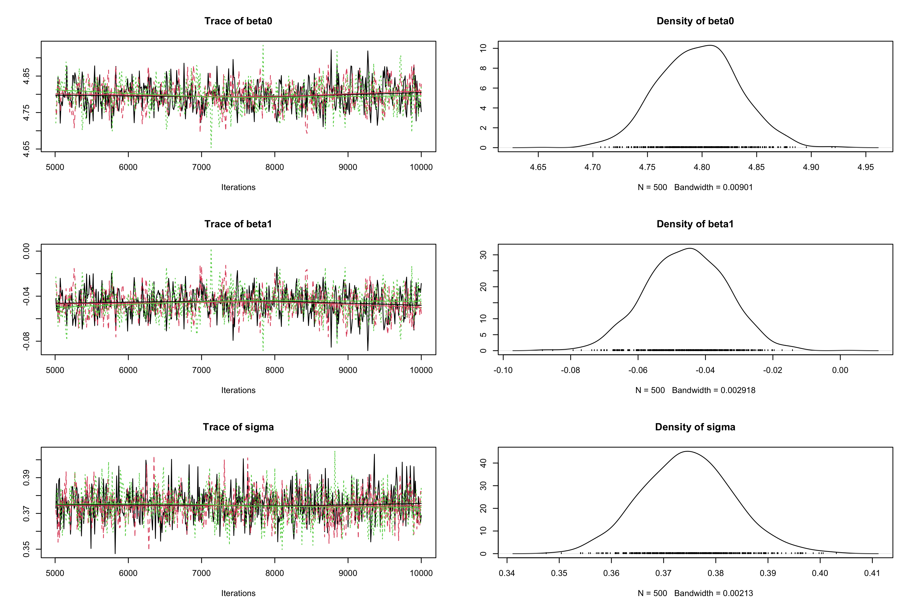

gelman.plot(res_albi_fixed_thin)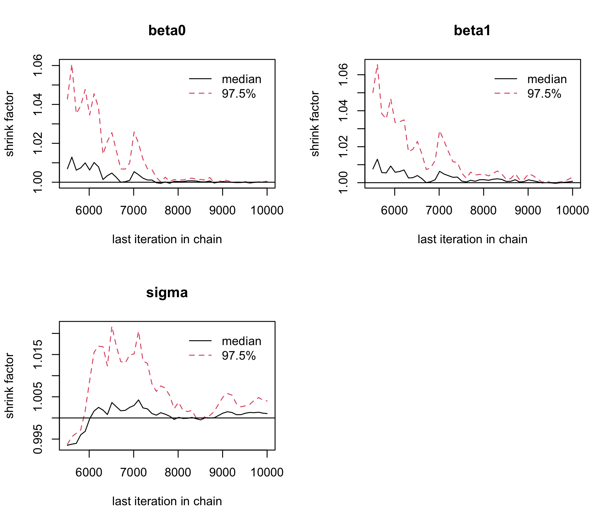

acfplot(res_albi_fixed_thin)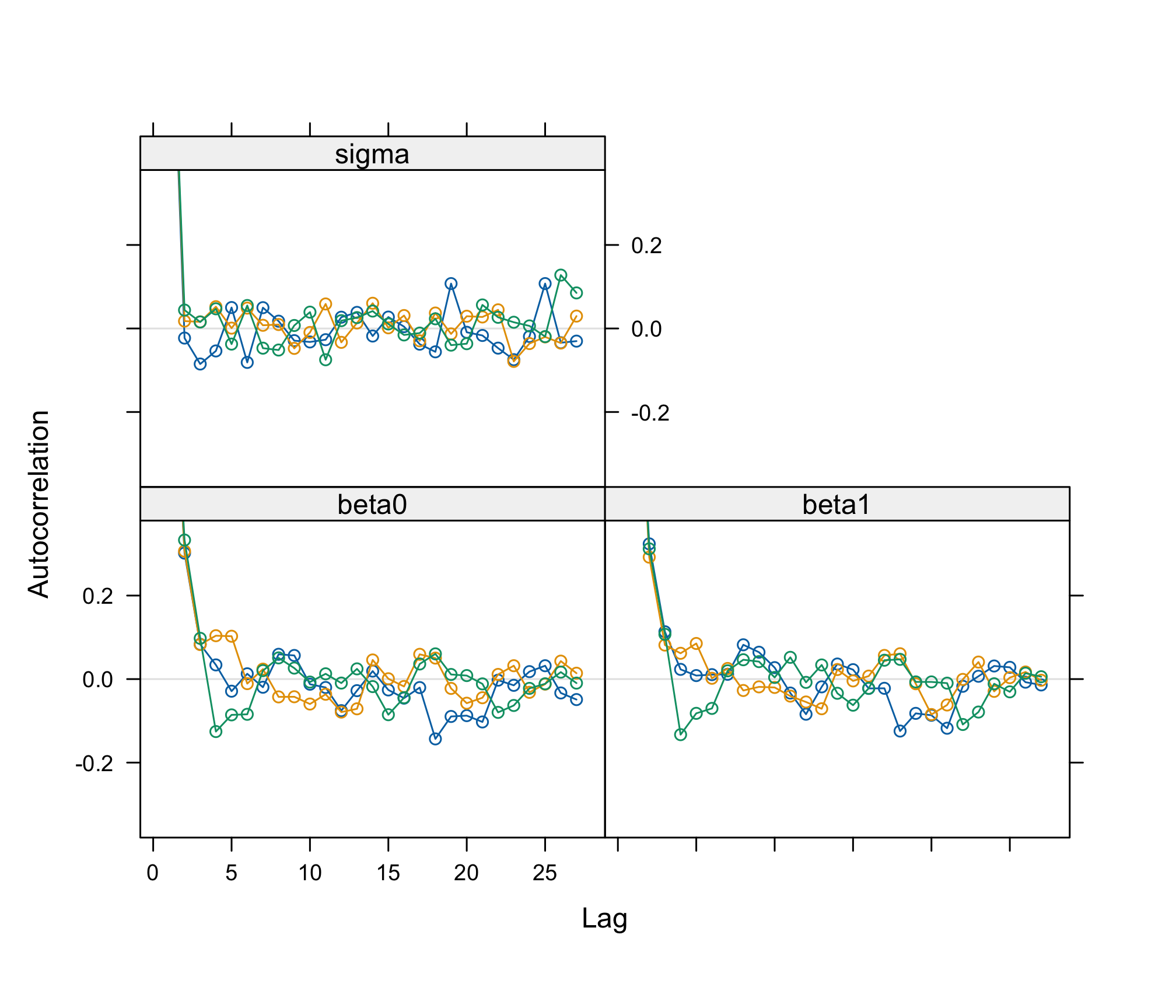

   par(mfrow=c(3, 3))
  cumuplot(res_albi_fixed_thin, ask=FALSE, auto.layout = FALSE)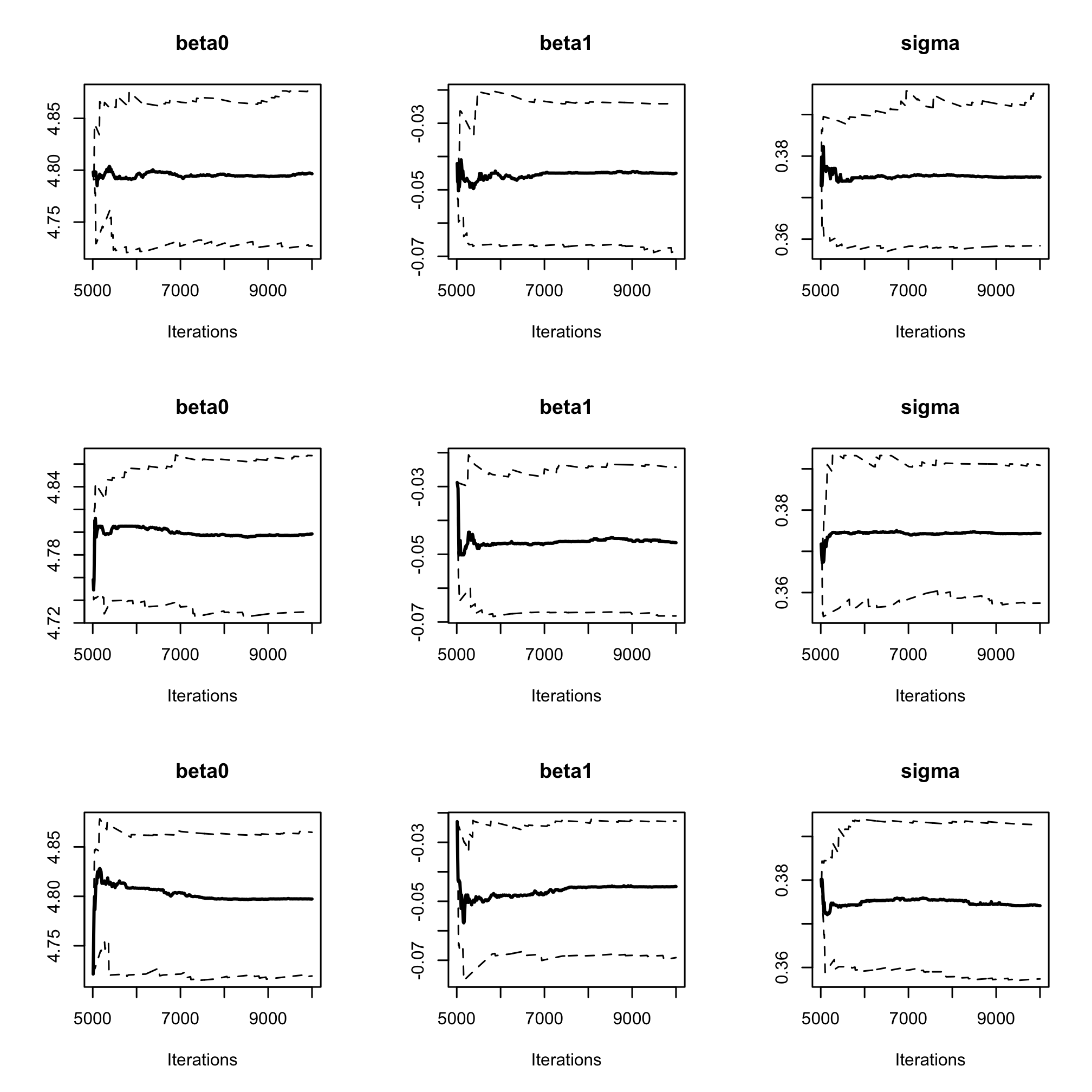

summary(res_albi_fixed_thin)

## 
## Iterations = 5010:10000
## Thinning interval = 10 
## Number of chains = 3 
## Sample size per chain = 500 
## 
## 1. Empirical mean and standard deviation for each variable,
##    plus standard error of the mean:
## 
##           Mean       SD  Naive SE Time-series SE
## beta0  4.79665 0.036241 0.0009357      0.0012446
## beta1 -0.04589 0.012045 0.0003110      0.0004101
## sigma  0.37458 0.008774 0.0002265      0.0002163
## 
## 2. Quantiles for each variable:
## 
##           2.5%      25%      50%      75%    97.5%
## beta0  4.72580  4.77043  4.79703  4.82106  4.86668
## beta1 -0.06845 -0.05394 -0.04618 -0.03814 -0.02216
## sigma  0.35791  0.36840  0.37465  0.37996  0.39314

Compare those results with a frequentist analysis.

  summary(lm(CD4t~ViralLoad, data=albi))

## 
## Call:
## lm(formula = CD4t ~ ViralLoad, data = albi)
## 
## Residuals:
##     Min      1Q  Median      3Q     Max 
## -1.0828 -0.2604 -0.0197  0.2449  1.3856 
## 
## Coefficients:
##             Estimate Std. Error t value Pr(>|t|)    
## (Intercept)  4.79635    0.03696   129.8  < 2e-16 ***
## ViralLoad   -0.04564    0.01201    -3.8 0.000154 ***
## ---
## Signif. codes:  0 '***' 0.001 '**' 0.01 '*' 0.05 '.' 0.1 ' ' 1
## 
## Residual standard error: 0.3742 on 948 degrees of freedom
## Multiple R-squared:  0.01501,	Adjusted R-squared:  0.01397 
## F-statistic: 14.44 on 1 and 948 DF,  p-value: 0.0001537

Perform a Bayesian logistic regression to study the impact of the treatment on the binary outcome CD4sup500 adjusted on the viral load. Once you have a first estimation, try adding an interaction between the treatment and the viral load.

# Fixed effect logistic regression Albi-ANRS
model{

  # likelihood
  for (i in 1:N){
    CD4sup500[i] ~ dbern(proba[i])
    logit(proba[i]) <- beta0 + beta1*VL[i] + beta2*Tt_switch[i] + beta3*d4t[i] + beta4*VL[i]*d4t[i] +         beta5*VL[i]*Tt_switch[i]
  }

  #Priors
  beta0~dnorm(0,0.0001)
  beta1~dnorm(0,0.0001)
  beta2~dnorm(0,0.0001)
  beta3~dnorm(0,0.0001)
  beta4~dnorm(0,0.0001)
  beta5~dnorm(0,0.0001)

  #ORs
  OR_VL <- exp(beta1)
  OR_switch <- exp(beta2)
  OR_d4t <- exp(beta3)
  OR_d4tVL <- exp(beta4)
  OR_swVL <- exp(beta5)
}

library(rjags)
albi_logis_jags <- jags.model("albiBUGSmodel_logistic_fixed.txt", 
                              data = list('CD4sup500' =  1*(albi$CD4sup500=="Yes"), 
                                          'N' = nrow(albi), 
                                          'VL' = albi$ViralLoad,
                                          'd4t' = 1*(albi$Treatment == "d4t+ddI"),
                                          'Tt_switch' = 1*(albi$Treatment == "switch")), 
                              n.chains = 3)

## Compiling model graph
##    Resolving undeclared variables
##    Allocating nodes
## Graph information:
##    Observed stochastic nodes: 950
##    Unobserved stochastic nodes: 6
##    Total graph size: 7299
## 
## Initializing model

res_albi_logis <- coda.samples(model = albi_logis_jags, 
                               variable.names = c('OR_VL', 'OR_switch', 'OR_d4t', 'OR_d4tVL', 'OR_swVL'), 
                               n.iter = 10000)
res_albi_logis_burnt <- window(res_albi_logis, start = 5001)

plot(res_albi_logis_burnt)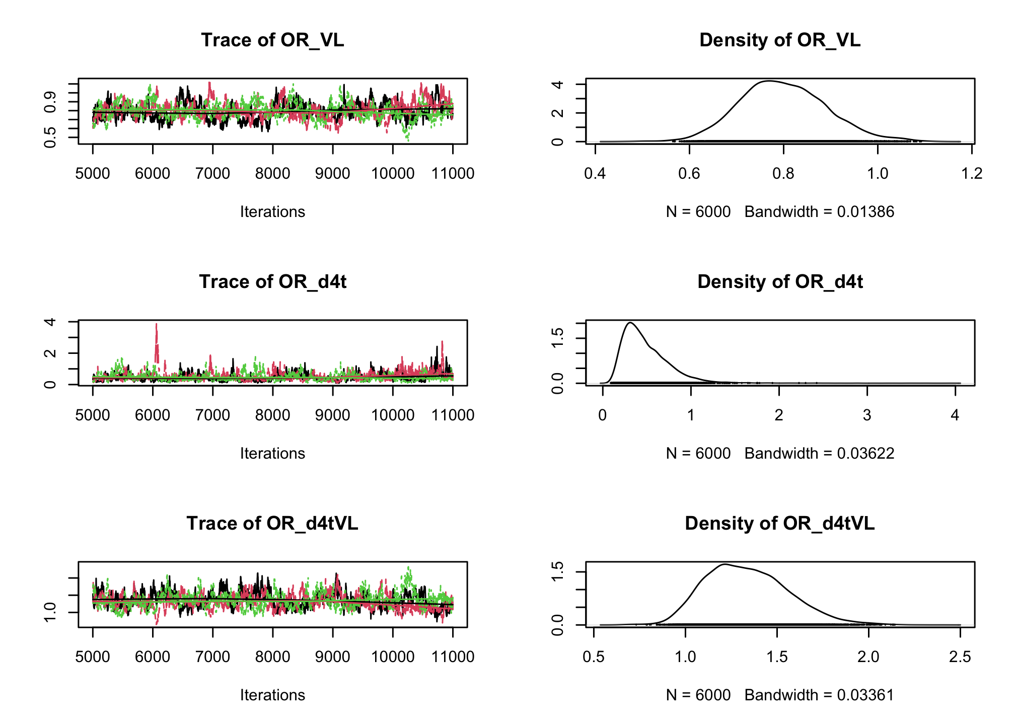

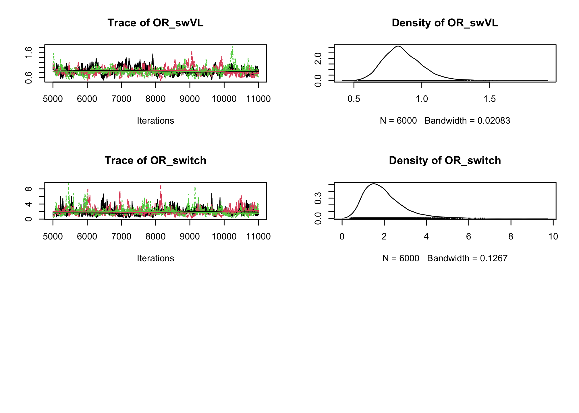
summary(res_albi_logis_burnt)

## 
## Iterations = 5001:11000
## Thinning interval = 1 
## Number of chains = 3 
## Sample size per chain = 6000 
## 
## 1. Empirical mean and standard deviation for each variable,
##    plus standard error of the mean:
## 
##             Mean      SD  Naive SE Time-series SE
## OR_VL     0.7769 0.09343 0.0006964       0.007154
## OR_d4t    0.4369 0.25163 0.0018755       0.017733
## OR_d4tVL  1.3978 0.24730 0.0018433       0.017420
## OR_swVL   0.8901 0.14784 0.0011019       0.008916
## OR_switch 1.8120 0.88270 0.0065793       0.053330
## 
## 2. Quantiles for each variable:
## 
##             2.5%    25%    50%   75%  97.5%
## OR_VL     0.5994 0.7131 0.7749 0.835 0.9736
## OR_d4t    0.1308 0.2629 0.3762 0.546 1.1008
## OR_d4tVL  0.9761 1.2257 1.3738 1.543 1.9445
## OR_swVL   0.6350 0.7857 0.8759 0.982 1.2144
## OR_switch 0.6469 1.1776 1.6391 2.252 4.0209

summary(glm(CD4sup500=="Yes"~ ViralLoad*Treatment, family="binomial", data=albi))

## 
## Call:
## glm(formula = CD4sup500 == "Yes" ~ ViralLoad * Treatment, family = "binomial", 
##     data = albi)
## 
## Coefficients:
##                            Estimate Std. Error z value Pr(>|z|)  
## (Intercept)                  0.3279     0.3241   1.012   0.3117  
## ViralLoad                   -0.2556     0.1197  -2.135   0.0328 *
## Treatmentd4t+ddI            -0.9409     0.5338  -1.763   0.0779 .
## Treatmentswitch              0.4836     0.4807   1.006   0.3143  
## ViralLoad:Treatmentd4t+ddI   0.3084     0.1737   1.776   0.0757 .
## ViralLoad:Treatmentswitch   -0.1303     0.1690  -0.771   0.4409  
## ---
## Signif. codes:  0 '***' 0.001 '**' 0.01 '*' 0.05 '.' 0.1 ' ' 1
## 
## (Dispersion parameter for binomial family taken to be 1)
## 
##     Null deviance: 1287.8  on 949  degrees of freedom
## Residual deviance: 1270.9  on 944  degrees of freedom
## AIC: 1282.9
## 
## Number of Fisher Scoring iterations: 4

So far we have ignored the longitudinal nature of our measurements. Now, lets add a random intercept in our logistic regression to account for the intra-patient correlation across visits.

ggplot(albi, aes(y = CD4, x = Day, color = Treatment)) +
  geom_hline(aes(yintercept=500), color="grey35", linetype = 2) + 
  geom_line(aes(group=PatientID), alpha=0.3) +
  MetBrewer::scale_color_met_d("Java") +
  theme_bw()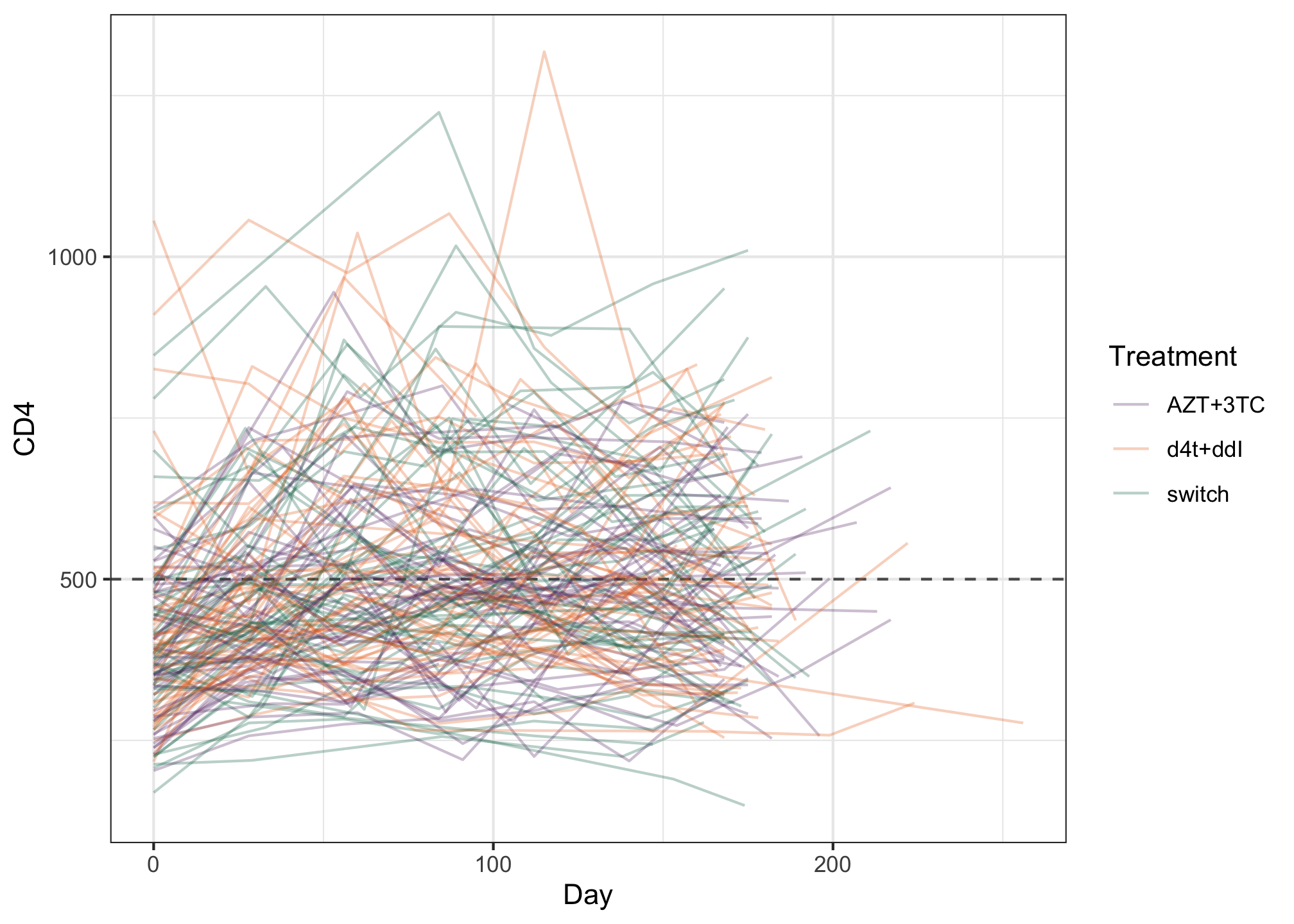

  # Mixed effect logistic regression Albi-ANRS
  model{

    # likelihood
    for (i in 1:N){
      CD4sup500[i] ~ dbern(proba[i])
      logit(proba[i]) <- beta0 + b0[PAT_ID[i]] + beta1*VL[i] + beta2*Tt_switch[i] + beta3*d4t[i] + beta4*VL[i]*d4t[i] +         beta5*VL[i]*Tt_switch[i]
    }

    for (j in 1:Npat){
      b0[j]~dnorm(0, tau_b0)
    }

    #Priors
    beta0~dnorm(0,0.0001)
    beta1~dnorm(0,0.0001)
    beta2~dnorm(0,0.0001)
    beta3~dnorm(0,0.0001)
    beta4~dnorm(0,0.0001)
    beta5~dnorm(0,0.0001)
    tau_b0~dgamma(0.001,0.001)

    #ORs
    OR_VL <- exp(beta1)
    OR_switch <- exp(beta2)
    OR_d4t <- exp(beta3)
    OR_d4tVL <- exp(beta4)
    OR_swVL <- exp(beta5)
    sigma_RI <- pow(tau_b0, -0.5)
  }

  library(rjags)
  albi_logis_RI_jags <- jags.model("albiBUGSmodel_logistic_RandomInt.txt", 
                                data = list('CD4sup500' =  1*(albi$CD4sup500=="Yes"), 
                                            'N' = nrow(albi), 
                                            'VL' = albi$ViralLoad,
                                            'd4t' = 1*(albi$Treatment == "d4t+ddI"),
                                            'Tt_switch' = 1*(albi$Treatment == "switch"),
                                            'Npat' = length(levels(albi$PatientID)),
                                            'PAT_ID' = as.numeric(albi$PatientID)), 
                                n.chains = 3)

## Compiling model graph
##    Resolving undeclared variables
##    Allocating nodes
## Graph information:
##    Observed stochastic nodes: 950
##    Unobserved stochastic nodes: 156
##    Total graph size: 8670
## 
## Initializing model

  res_albi_logis_RI <- coda.samples(model = albi_logis_RI_jags, 
                                 variable.names = c('OR_VL', 'OR_switch', 'OR_d4t', 'OR_d4tVL', 'OR_swVL', 'sigma_RI'), 
                                 n.iter = 10000)
  res_albi_logis_RI_burnt <- window(res_albi_logis_RI, start = 1001)

  plot(res_albi_logis_RI_burnt)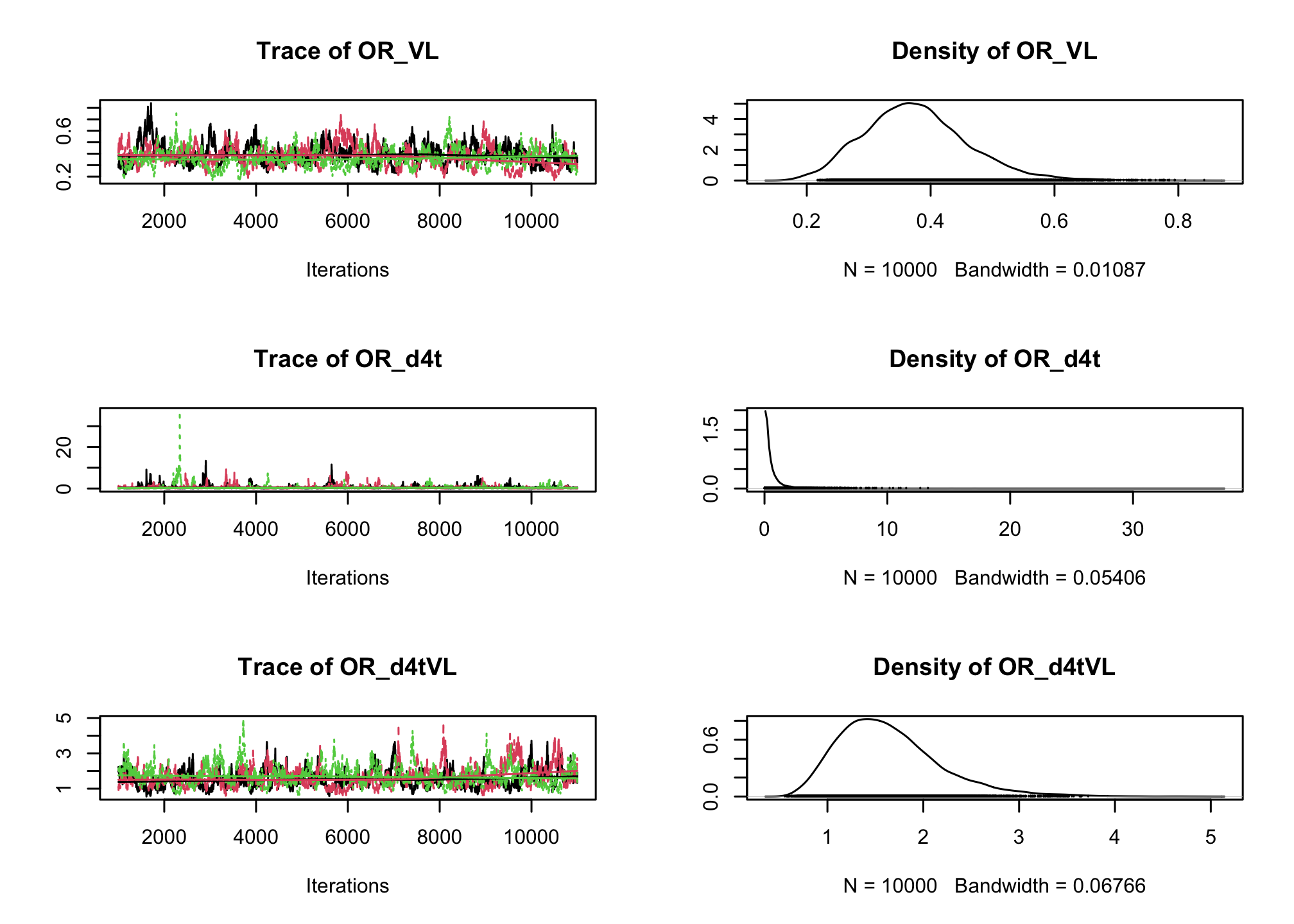

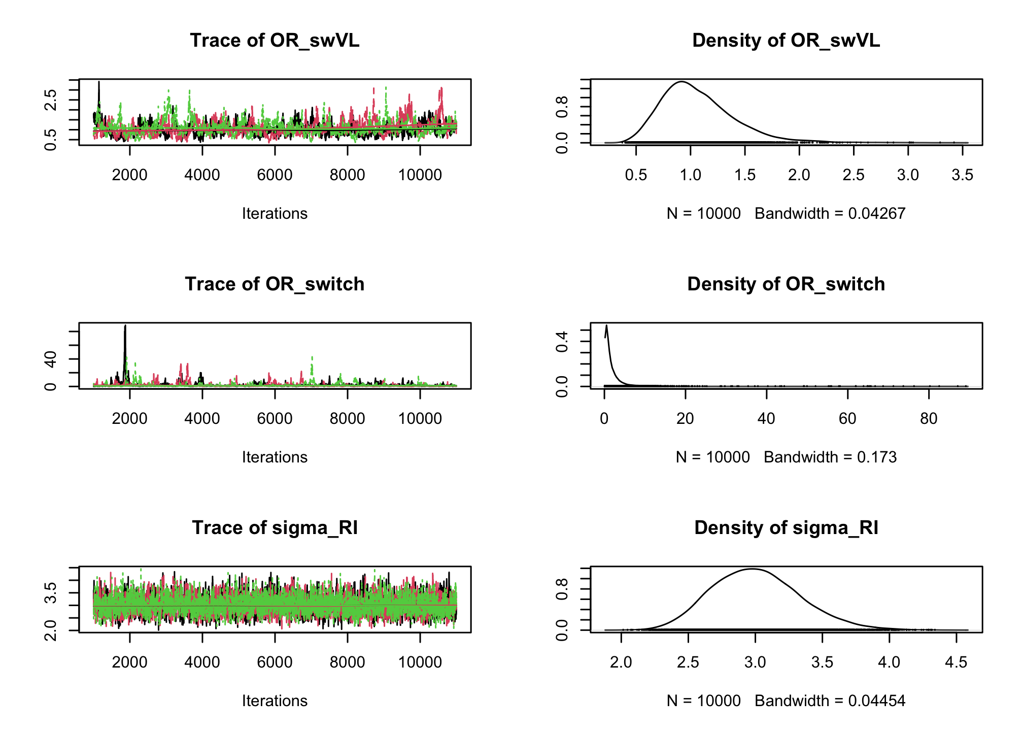
  summary(res_albi_logis_RI_burnt)

## 
## Iterations = 1001:11000
## Thinning interval = 1 
## Number of chains = 3 
## Sample size per chain = 10000 
## 
## 1. Empirical mean and standard deviation for each variable,
##    plus standard error of the mean:
## 
##             Mean      SD Naive SE Time-series SE
## OR_VL     0.3844 0.08452 0.000488       0.005470
## OR_d4t    0.6507 0.92448 0.005337       0.050909
## OR_d4tVL  1.5827 0.49078 0.002834       0.028619
## OR_swVL   1.0425 0.31646 0.001827       0.017970
## OR_switch 1.9475 2.39980 0.013855       0.130034
## sigma_RI  2.9970 0.33150 0.001914       0.006525
## 
## 2. Quantiles for each variable:
## 
##              2.5%    25%    50%    75%  97.5%
## OR_VL     0.24056 0.3218 0.3774 0.4404 0.5632
## OR_d4t    0.03959 0.1645 0.3435 0.7405 3.2864
## OR_d4tVL  0.80968 1.2284 1.5236 1.8690 2.7098
## OR_swVL   0.57400 0.8039 0.9975 1.2314 1.7848
## OR_switch 0.17300 0.5886 1.1918 2.3944 8.2116
## sigma_RI  2.41748 2.7637 2.9740 3.2026 3.7077

  library(lme4)
  summary(lme4::glmer(CD4sup500=="Yes"~ (1|PatientID) + ViralLoad*Treatment, family="binomial", data=albi))

## Generalized linear mixed model fit by maximum likelihood (Laplace
##   Approximation) [glmerMod]
##  Family: binomial  ( logit )
## Formula: CD4sup500 == "Yes" ~ (1 | PatientID) + ViralLoad * Treatment
##    Data: albi
## 
##       AIC       BIC    logLik -2*log(L)  df.resid 
##     971.8    1005.8    -478.9     957.8       943 
## 
## Scaled residuals: 
##     Min      1Q  Median      3Q     Max 
## -2.9273 -0.4021 -0.1947  0.4119  3.9688 
## 
## Random effects:
##  Groups    Name        Variance Std.Dev.
##  PatientID (Intercept) 7.317    2.705   
## Number of obs: 950, groups:  PatientID, 149
## 
## Fixed effects:
##                             Estimate Std. Error z value Pr(>|z|)    
## (Intercept)                 1.901075   0.689952   2.755  0.00586 ** 
## ViralLoad                  -0.955590   0.212725  -4.492 7.05e-06 ***
## Treatmentd4t+ddI           -1.177377   1.103323  -1.067  0.28592    
## Treatmentswitch             0.101717   1.000232   0.102  0.91900    
## ViralLoad:Treatmentd4t+ddI  0.439794   0.308829   1.424  0.15443    
## ViralLoad:Treatmentswitch   0.008679   0.291172   0.030  0.97622    
## ---
## Signif. codes:  0 '***' 0.001 '**' 0.01 '*' 0.05 '.' 0.1 ' ' 1
## 
## Correlation of Fixed Effects:
##             (Intr) VirlLd Trt4+I Trtmnt VL:T4+
## ViralLoad   -0.780                            
## Trtmntd4t+I -0.616  0.473                     
## Trtmntswtch -0.679  0.521  0.423              
## VrlLd:Tr4+I  0.518 -0.657 -0.821 -0.355       
## VrlLd:Trtmn  0.549 -0.695 -0.341 -0.786  0.475

Jean-Michel Molina et al. “The ALBI Trial: A Randomized Controlled Trial Comparing Stavudine Plus Didanosine with Zidovudine Plus Lamivudine and a Regimen Alternating Both Combinations in Previously Untreated Patients Infected with Human Immunodeficiency Virus,” The Journal of Infectious Diseases 180, no. 2 (1999): 351–358, doi:10.1086/314891.↩︎

Last updated on June 18, 2025

Edit this page