Exercise 6: Post-mortem analysis of an under-powered randomized trial

The randomized clinical trial EOLIA¹ evaluated a new treatment for severe acute respiratory distress syndrome (severe ARDS) by comparing the mortality rate after 60 days among 249 patients randomized between a control group (receiving conventional treatment, i.e. mechanical ventilation) and a treatment group receiving extracorporeal membrane oxygenation (ECMO) — the new treatment studied. A frequentist analysis of the data concluded to a Relative Risk of death of $0.76$ in the ECMO group compared to controls (in Intention to Treat), with $C I_{95 %} = [0.55, 1.04]$ and the associated p-value of $0.09$ .

Goligher et al. (2019) ² performed a Bayesian re-analysis of these data, further exploring the evidence and how it can be quantified and summarized with a Bayesian approach.

Observed data from the *EOLIA* trial
	Control	ECMO
$n$ observed	125	124
number of deceased at 60 days	57	44

Write the Bayesian model used by Goligher et al. (2019).

I) Question of interest:
Is the Relative Risk of death under ECMO compared to the conventional mechanical treatment less than one ?

II) Sampling model:
Let $Z_{c o n t r o l}$ be the number of death in the control group, and $Z_{e c m o}$ the number of death in the ECMO group $Z_{c o n t r o l} \sim B i n o m i a l (p_{c}, 125)$ $Z_{e c m o} \sim B i n o m i a l (R R \times p_{c}, 124)$
III) Priors: $p_{c} \sim U_{[0, 1]}$ $l o g (R R) \sim U_{[- 17, 17]}$
NB: $U_{[- 17, 17]}$ has approximately a standard deviation of 10 (cf Table 1 and Figure 2.A – orange lines – of Goligher et al., 2019³)
NB: One can also define a sampling model at the individual level:
Let $Y_{c o n t r o l_{i}}$ be a binary variable indicating whether the patient $i$ from the control group died before 60 days, and $Y_{e c m o_{i}}$ a similar variable for patient from the ecmo group. $Y_{c o n t r o l_{i}} \overset{i i d}{\sim} B e r n o u l l i (p_{c})$ $Y_{e c m o_{i}} \overset{i i d}{\sim} B e r n o u l l i (R R \times p_{c})$

Write the corresponding BUGS model, and save it into a .txt file (for instance called goligherBUGSmodel.txt)

As we have seen above, there are two equivalent ways of defining the sampling model:

either at the population level with a Binomial likelihood,
or at the individual level with a Bernoulli likelihood

# Population model
model{

  # Sampling model
  zcontrol~dbin(pc, ncontrol)
  zecmo~dbin(RR*pc, necmo)

  # Prior
  logRR~dunif(-17, 17) # SD is approximately 10
  pc~dunif(0,1) #probability of death in the control group

  # Re-parameterizations
  RR <- exp(logRR)
  ARR <- pc - RR*pc
}

# Individual model
model{

  # Sampling model
  for (i in 1:ncontrol){
    ycontrol[i]~dbern(pc)
  }
  for (i in 1:necmo){
    yecmo[i]~dbern(RR*pc)
  }

  # Prior
  logRR~dunif(-17, 17) # SD is approximately 10
  pc~dunif(0,1) #probability of death in the control group

  # Re-parameterizations
  RR <- exp(logRR)
  ARR <- pc - RR*pc
}

First create two binary data vectors ycontrol and yecmo (or ycontrol and yecmo that are either 1 or 0, using the rep() R function if you prefer the individual model), to encode the observations from the data table above. Then uses the jags.model() and coda.samples() to replicate the estimation from Goligher et al. (2019) (ProTip: use the function window() to remove the burn-in observation from the output of the coda.samples function.)

#Individual data
ncontrol <- 125
zcontrol <- 57
ycontrol <- c(rep(1, zcontrol), rep(0, ncontrol-zcontrol))

necmo <- 124
zecmo <- 44
yecmo <- c(rep(1, zecmo), rep(0, necmo-zecmo))


#Population data model
#sampling
library(rjags)
goligher_jags_pop <- jags.model(file = "goligherBUGSmodel_pop.txt", 
                                  data = list("zcontrol" =  zcontrol, 
                                              "ncontrol" = ncontrol,
                                              "zecmo" =  zecmo, 
                                              "necmo" = necmo
                                              ), 
                                  n.chains = 3)

## Compiling model graph
##    Resolving undeclared variables
##    Allocating nodes
## Graph information:
##    Observed stochastic nodes: 2
##    Unobserved stochastic nodes: 2
##    Total graph size: 13
## 
## Initializing model

res_goligher_pop <- coda.samples(model = goligher_jags_pop, 
                                       variable.names = c('pc', 'RR', 'ARR'), 
                                       n.iter = 40000)

#post-processing
res_goligher_burnt_pop <- window(res_goligher_pop, start=21001) # removes burn-in for Markov chain convergence
#NB: by default coda.samples() performs 1000 first burnin iterations that are automatically removed from the output but still indexed.

#Individual data model

goligher_jags_indiv <- jags.model(file = "goligherBUGSmodel_indiv.txt", 
                                  data = list("ycontrol" =  ycontrol, 
                                              "ncontrol" = ncontrol,
                                              "yecmo" =  yecmo, 
                                              "necmo" = necmo
                                              ), 
                                  n.chains = 3)

## Compiling model graph
##    Resolving undeclared variables
##    Allocating nodes
## Graph information:
##    Observed stochastic nodes: 249
##    Unobserved stochastic nodes: 2
##    Total graph size: 260
## 
## Initializing model

res_goligher_indiv <- coda.samples(model = goligher_jags_indiv, 
                                       variable.names = c('pc', 'RR', 'ARR'), 
                                       n.iter = 40000)

#postprocessing
res_goligher_burnt_indiv <- window(res_goligher_indiv, start=21001) # removes burn-in for Markov chain convergence

Check the convergence, and then comment the estimate results (ProTip: look at the effective sample size with the effectiveSize() function).

effectiveSize(res_goligher_burnt_pop)

##      ARR       RR       pc 
## 15319.12 16491.33 16416.42

plot(res_goligher_burnt_pop)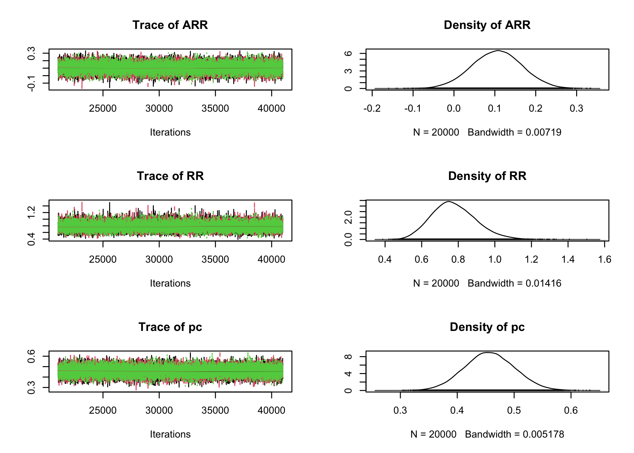

gelman.plot(res_goligher_burnt_pop)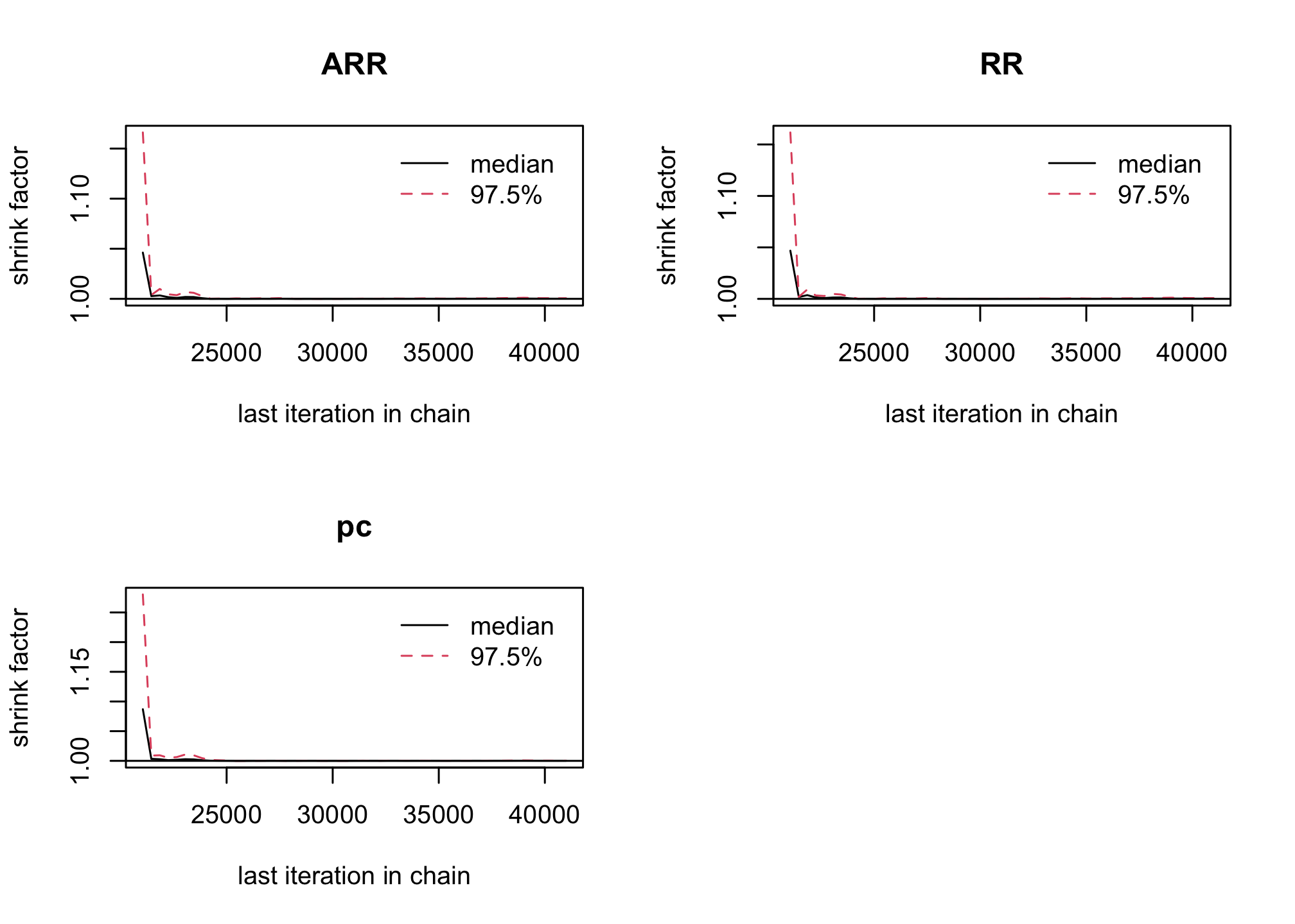

acfplot(res_goligher_burnt_pop)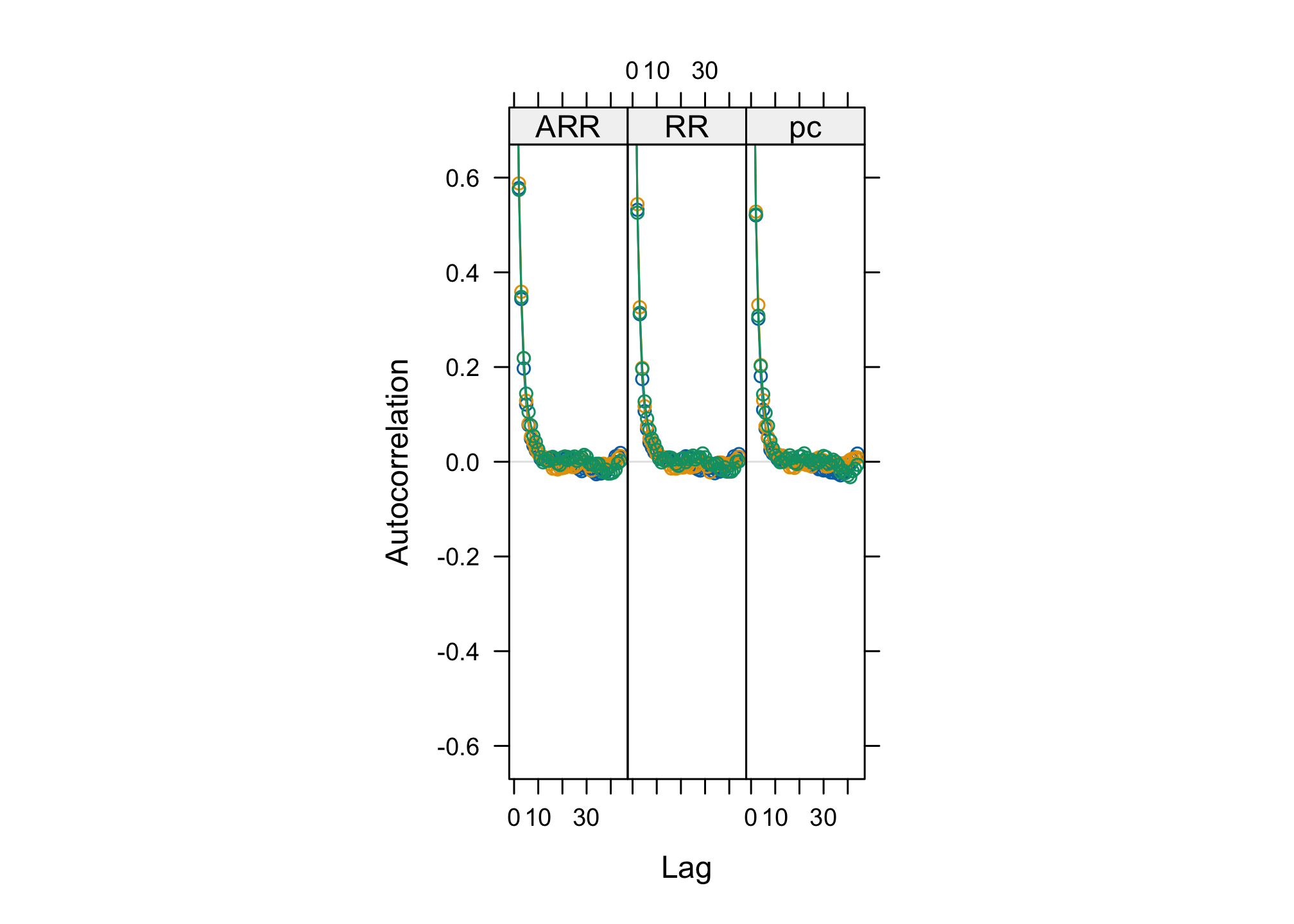

par(mfrow=c(3, 2))
cumuplot(res_goligher_burnt_pop, ask=FALSE, auto.layout = FALSE)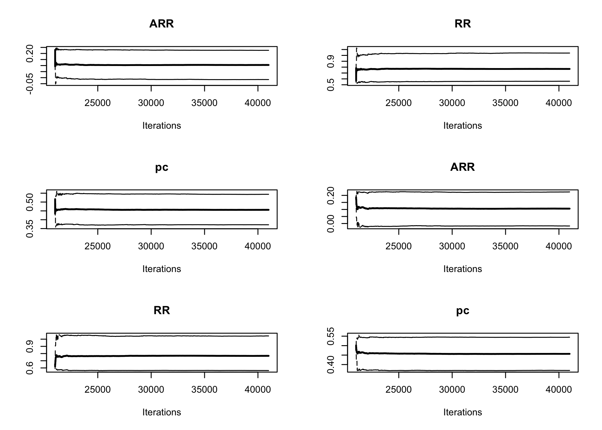

par(mfrow=c(1, 1))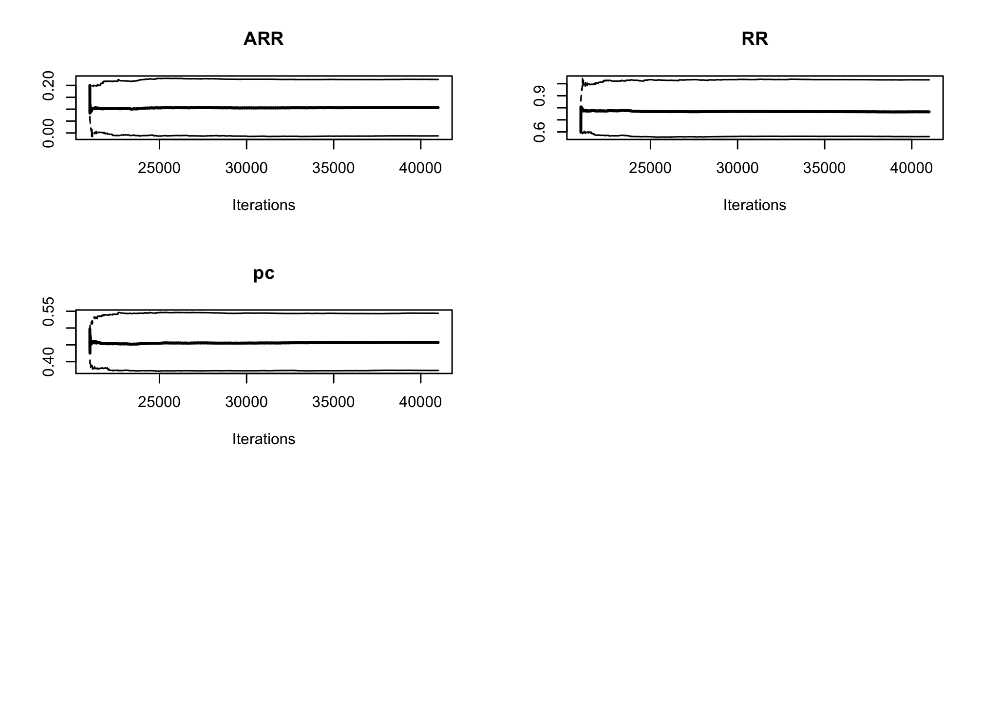

summary(res_goligher_burnt_pop)

## 
## Iterations = 21001:41000
## Thinning interval = 1 
## Number of chains = 3 
## Sample size per chain = 20000 
## 
## 1. Empirical mean and standard deviation for each variable,
##    plus standard error of the mean:
## 
##       Mean      SD  Naive SE Time-series SE
## ARR 0.1046 0.06106 0.0002493      0.0004933
## RR  0.7783 0.12153 0.0004961      0.0009463
## pc  0.4568 0.04392 0.0001793      0.0003431
## 
## 2. Quantiles for each variable:
## 
##         2.5%     25%    50%    75%  97.5%
## ARR -0.01536 0.06334 0.1051 0.1463 0.2231
## RR   0.56368 0.69251 0.7700 0.8547 1.0388
## pc   0.37172 0.42679 0.4563 0.4866 0.5432

summary(res_goligher_burnt_indiv)

## 
## Iterations = 21001:41000
## Thinning interval = 1 
## Number of chains = 3 
## Sample size per chain = 20000 
## 
## 1. Empirical mean and standard deviation for each variable,
##    plus standard error of the mean:
## 
##       Mean      SD  Naive SE Time-series SE
## ARR 0.1042 0.06177 0.0002522      0.0005082
## RR  0.7792 0.12318 0.0005029      0.0009769
## pc  0.4562 0.04432 0.0001809      0.0003500
## 
## 2. Quantiles for each variable:
## 
##         2.5%     25%    50%    75%  97.5%
## ARR -0.01769 0.06246 0.1043 0.1463 0.2245
## RR   0.56165 0.69298 0.7708 0.8565 1.0447
## pc   0.37039 0.42615 0.4560 0.4862 0.5437

# shortest 95% Credibility interval:
HDInterval::hdi(res_goligher_burnt_pop)

##               ARR       RR        pc
## lower -0.01417227 0.550152 0.3716910
## upper  0.22407131 1.020956 0.5431143
## attr(,"credMass")
## [1] 0.95

# posterior porbability of RR <1: (answering our question !)
head(res_goligher_burnt_pop[[1]]) # first chain

## Markov Chain Monte Carlo (MCMC) output:
## Start = 21001 
## End = 21007 
## Thinning interval = 1 
##             ARR        RR        pc
## [1,] 0.14318628 0.7120283 0.4972234
## [2,] 0.10948919 0.7378604 0.4176751
## [3,] 0.09960137 0.7659285 0.4255168
## [4,] 0.10253812 0.7805459 0.4672417
## [5,] 0.08653039 0.7883640 0.4088643
## [6,] 0.03088816 0.9246668 0.4100206
## [7,] 0.07224484 0.8197520 0.4008080

head(res_goligher_burnt_pop[[2]]) # second chain

## Markov Chain Monte Carlo (MCMC) output:
## Start = 21001 
## End = 21007 
## Thinning interval = 1 
##             ARR        RR        pc
## [1,] 0.14158471 0.6984512 0.4695250
## [2,] 0.08839096 0.7953862 0.4319891
## [3,] 0.14258264 0.7095738 0.4909427
## [4,] 0.17152840 0.6202759 0.4517185
## [5,] 0.10648208 0.7553651 0.4352694
## [6,] 0.13298879 0.6802404 0.4159024
## [7,] 0.00791193 0.9797028 0.3898039

mean(c(sapply(res_goligher_burnt_pop, "[", , "RR"))<1)

## [1] 0.9555333

Change to a more informative prior using a Gaussian distribution for the log(RR), centered on log(0.78) and with a standard deviation of 0.15 in the log(RR) scale (i.e. a precision of $\approx 45$ ). Comment the results. Try out other prior distributions.
```
1/(0.15^2)
```
```
## [1] 44.44444
```
```
 logRR~dnorm(log(0.78), 45)
```

Alain Combes et al. “Extracorporeal Membrane Oxygenation for Severe Acute Respiratory Distress Syndrome,” New England Journal of Medicine 378, no. 21 (2018): 1965–1975, doi:10.1056/NEJMoa1800385.↩︎
Ewan C. Goligher et al. “Extracorporeal Membrane Oxygenation for Severe Acute Respiratory Distress Syndrome and Posterior Probability of Mortality Benefit in a Post Hoc Bayesian Analysis of a Randomized Clinical Trial,” JAMA 320, no. 21 (2018): 2251, doi:10.1001/jama.2018.14276.↩︎
Goligher et al. “Extracorporeal Membrane Oxygenation for Severe Acute Respiratory Distress Syndrome and Posterior Probability of Mortality Benefit in a Post Hoc Bayesian Analysis of a Randomized Clinical Trial”.↩︎

Last updated on June 18, 2025

Edit this page