Exercise 7: Bayesian meta-analysis

In 2014, Crins et al. ¹ published a meta-analysis assessing the incidence of acute rejection (AR) with or without Interleukin-2 receptor antagonists. In this exercise we will recreate this analysis.

Load the package bayesmeta ² and the data from Crins et al. (2014) with the R command data("CrinsEtAl2014").
```
library(bayesmeta)
data(CrinsEtAl2014)
```
Play around with the companion shiny app at: https://rshiny.gwdg.de/apps/bayesmeta/.
If the website is unavailable, you can launch the app locally by running the 2 following commands from :
```
library("shiny")
install.packages("rhandsontable")
runUrl("https://wwwuser.gwdg.de/~croever/bayesmeta/bayesmeta-app.zip")
```

Directly in the console now, using the escalc() function from the package metafor, compute the estimated log odds ratios from the 6 considered studies alongside their sampling variances (ProTip: read the Measures for Dichotomous Variables section from the help of the escalc() function). Check that those are the same as the one on the online shiny app (ProTip: ‘sigma’ is the standard error, i.e. the square root of the sampling variance vi)

library("metafor")
crins.es <- escalc(measure="OR",
                   ai=exp.AR.events,  n1i=exp.total,
                   ci=cont.AR.events, n2i=cont.total,
                   slab=publication, data=CrinsEtAl2014)
crins.es[,c("publication", "yi", "vi")]

publication	yi	vi
Heffron (2003)	-2.3097026	0.3593718
Gibelli (2004)	-0.4595323	0.3095760
Schuller (2005)	-2.3025851	0.7750000
Ganschow (2005)	-1.7578579	0.2078161
Spada (2006)	-1.2584610	0.4121591
Gras (2008)	-2.4178959	2.3372623

NB: Log-odds ratios are symmetric around zero and have a sampling distribution closer to the normal distibution than the natural OR scale. For this reason, they are usually prefered for meta-analyses. Their sample variance is then computed as the sum of the inverse of all the counts in the $2 \times 2$ associated contingency table³.

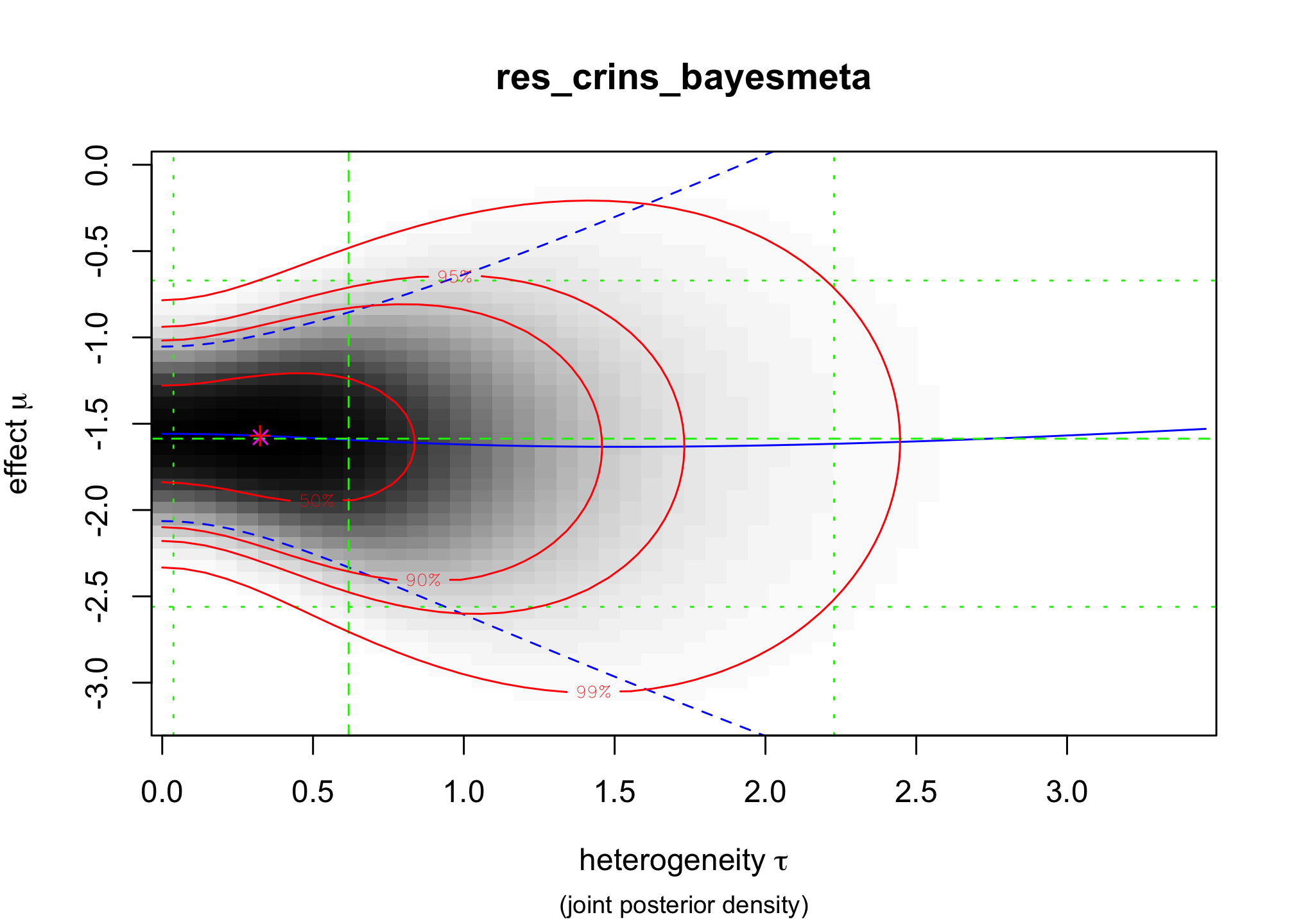
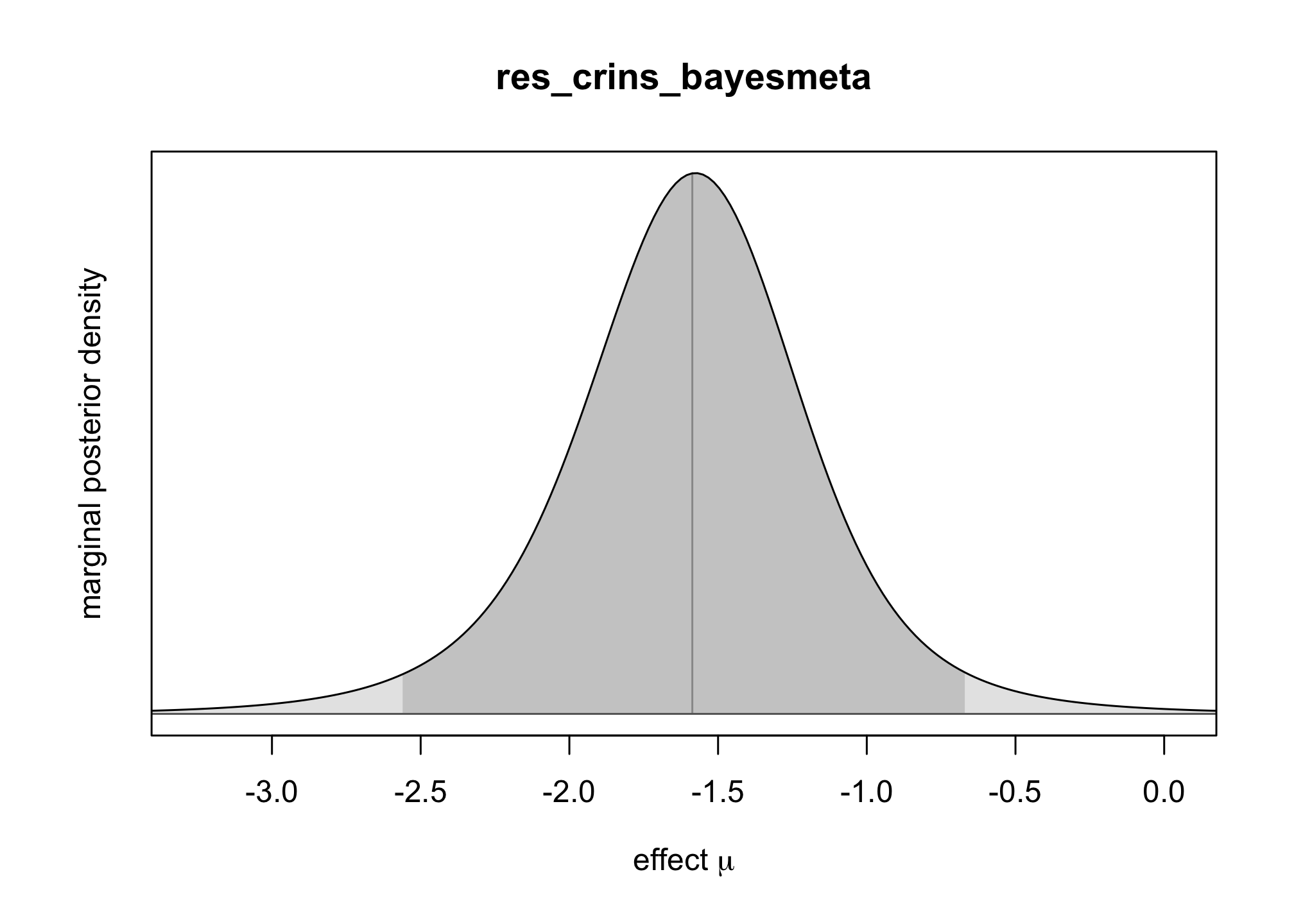
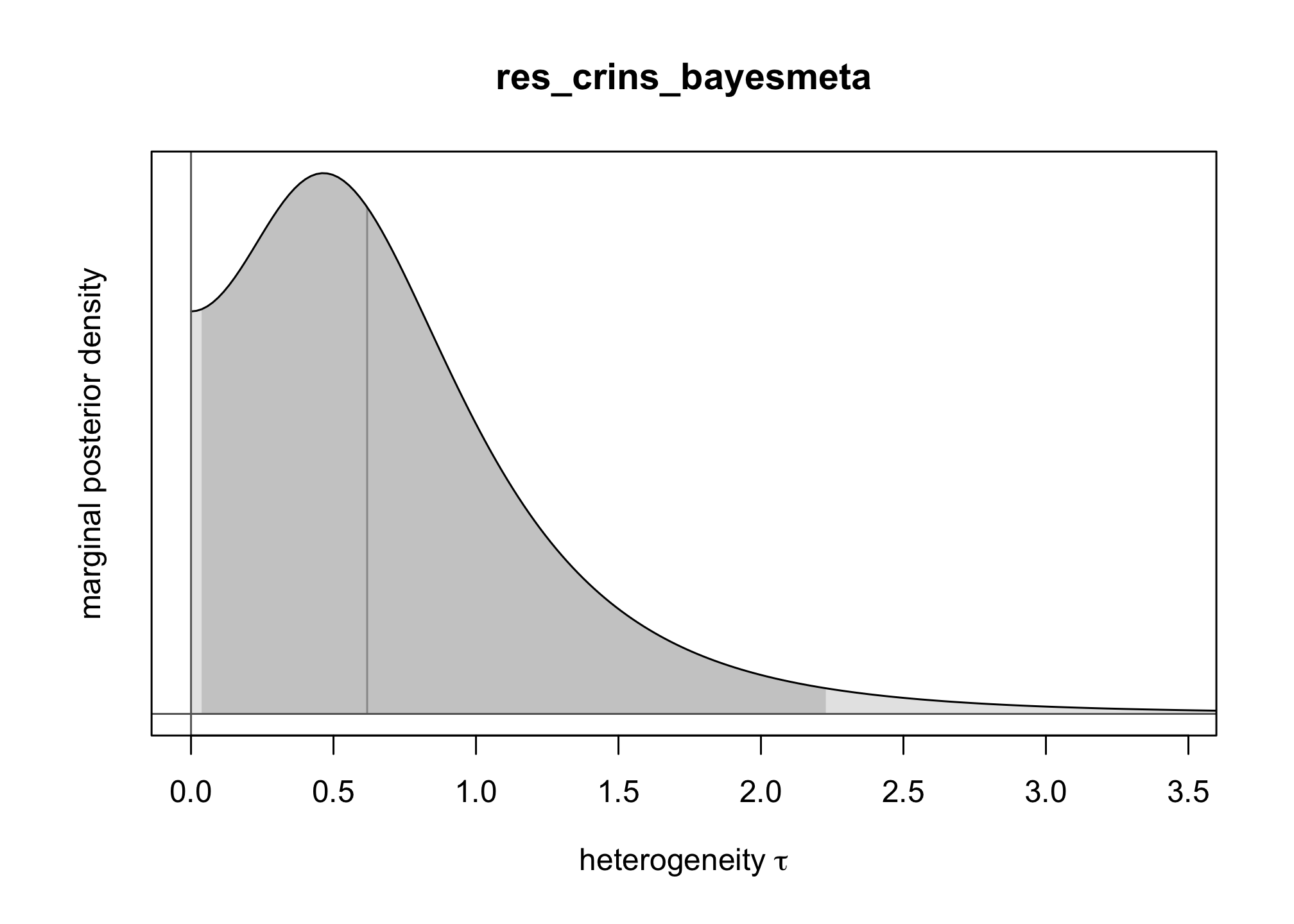
Perform a random-effect meta-analysis of those data using the bayesmeta() function from the package bayesmeta, within . Use a uniform prior on $[0, 4]$ for $τ$ and a Gaussian prior for $μ$ centered around $0$ and with a standard deviation of $4$ .

res_crins_bayesmeta <- bayesmeta(y=crins.es$yi, sigma=sqrt(crins.es$vi), 
                                 labels=crins.es$publication,
                                 tau.prior = function(t){dunif(t, max=4)},
                                 mu.prior = c(0, 4),
                                 interval.type = "central")
summary(res_crins_bayesmeta)

##  'bayesmeta' object.
## data (6 estimates):
##                          y     sigma
## Heffron (2003)  -2.3097026 0.5994763
## Gibelli (2004)  -0.4595323 0.5563956
## Schuller (2005) -2.3025851 0.8803408
## Ganschow (2005) -1.7578579 0.4558685
## Spada (2006)    -1.2584610 0.6419962
## Gras (2008)     -2.4178959 1.5288107
## 
## tau prior (proper):
## function (t) 
## {
##     dunif(t, max = 4)
## }
## <bytecode: 0x127edc9a8>
## 
## mu prior (proper):
## normal(mean=0, sd=4)
## 
## ML and MAP estimates:
##                    tau        mu
## ML joint     0.3258895 -1.578317
## ML marginal  0.4644136 -1.587347
## MAP joint    0.3244300 -1.569497
## MAP marginal 0.4644205 -1.576092
## 
## marginal posterior summary:
##                  tau         mu      theta
## mode      0.46442045 -1.5760916 -1.5656380
## median    0.61810119 -1.5866193 -1.5806176
## mean      0.73768542 -1.5935568 -1.5935568
## sd        0.56879971  0.4698241  1.0448965
## 95% lower 0.03724555 -2.5605641 -3.7989794
## 95% upper 2.22766946 -0.6704235  0.5580817
## 
## (quoted intervals are central, equal-tailed credible intervals.)
## 
## Bayes factors:
##             tau=0        mu=0
## actual  2.6800815 0.094852729
## minimum 0.7442665 0.008342187
## 
## relative heterogeneity I^2 (posterior median): 0.4718317

plot(res_crins_bayesmeta)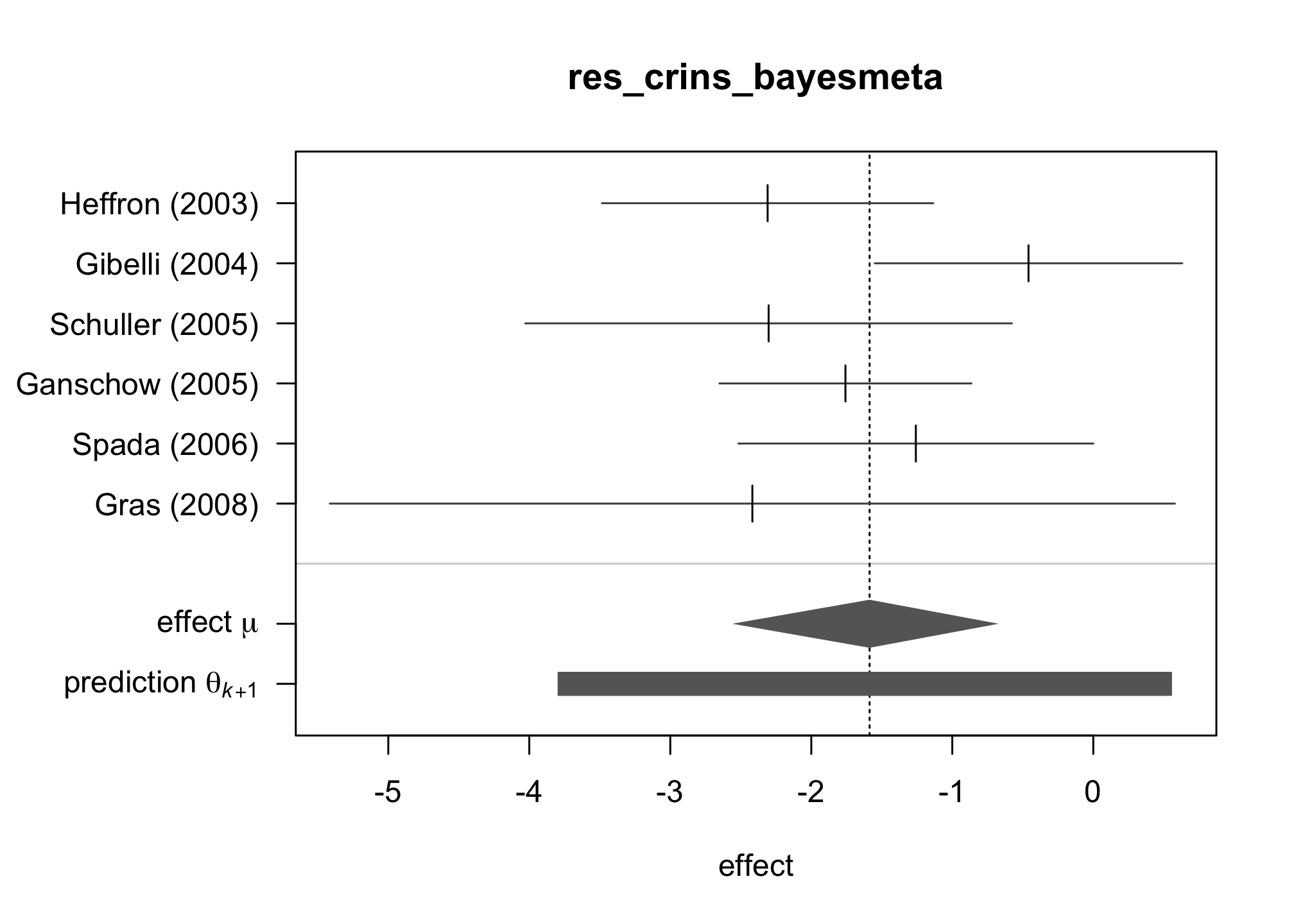

Write the corresponding random-effects Bayesian meta-analysis model (using math, not – yet).

I) Question of interest:
Is the treatment (IL2RA) odds ratio for Acute Rejection events inferior to 1 ?
II) Sampling model:
Let $y_{i}$ be the log-odds-ratio reported by the study $i$ and $σ_{i}^{2}$ its sampling variance $y_{i} \overset{i i d}{\sim} N (θ_{i}, σ_{i}^{2})$ $θ_{i} \overset{i i d}{\sim} N (μ, τ^{2})$ III) Priors: $θ_{i} \overset{i i d}{\sim} N (μ, τ^{2})$ $μ \sim N (0, 4^{2})$ $τ \sim U_{[0, 4]}$

Use rjags to estimate the same model, saving the BUGS model in a .txt file (called crinsBUGSmodel.txt for instance).

# Random-effects model for Crins et al. 2014 Acute Rejection meta-analysis
model{

  # Sampling model/likelihood
  for (i in 1:N){
    logOR[i]~dnorm(theta[i], precision.logOR[i])
  }

  # Priors
  for (i in 1:N){
    theta[i]~dnorm(mu, precision.tau)
  }
  mu~dnorm(0, 0.0625) # 1/16 = 0.0625
  tau~dunif(0, 4)

  # Re-parameterization
  for(i in 1:N){
    precision.logOR[i] <- pow(sigma[i], -2)
  }
  precision.tau <- pow(tau, -2)
  OR <- exp(mu)
}

# Sampling
library(rjags)
crins_jags_res <- jags.model(file = "crinsBUGSmodel.txt", 
                                  data = list("logOR" =  crins.es$yi,
                                              "sigma" = sqrt(crins.es$vi),
                                              "N" = length(crins.es$yi)
                                              ), 
                                  n.chains = 3)

## Compiling model graph
##    Resolving undeclared variables
##    Allocating nodes
## Graph information:
##    Observed stochastic nodes: 6
##    Unobserved stochastic nodes: 8
##    Total graph size: 34
## 
## Initializing model

res_crins_jags_res <- coda.samples(model = crins_jags_res, 
                                       variable.names = c("mu", "tau", "OR"), 
                                       n.iter = 20000)

# Postprocessing
res_crins_jags_res <- window(res_crins_jags_res, start=5001) # remove burn-in for Markov chain convergence
summary(res_crins_jags_res)

## 
## Iterations = 5001:21000
## Thinning interval = 1 
## Number of chains = 3 
## Sample size per chain = 16000 
## 
## 1. Empirical mean and standard deviation for each variable,
##    plus standard error of the mean:
## 
##        Mean     SD  Naive SE Time-series SE
## OR   0.2289 0.1749 0.0007983       0.001300
## mu  -1.5972 0.4763 0.0021740       0.004006
## tau  0.7536 0.5737 0.0026185       0.010510
## 
## 2. Quantiles for each variable:
## 
##        2.5%     25%     50%    75%   97.5%
## OR   0.0773  0.1558  0.2032  0.264  0.5168
## mu  -2.5601 -1.8592 -1.5935 -1.332 -0.6601
## tau  0.0394  0.3501  0.6339  1.010  2.2454

HDInterval::hdi(res_crins_jags_res)

##               OR         mu          tau
## lower 0.04670089 -2.5433691 0.0001443916
## upper 0.43440863 -0.6474327 1.8469964221
## attr(,"credMass")
## [1] 0.95

plot(res_crins_jags_res)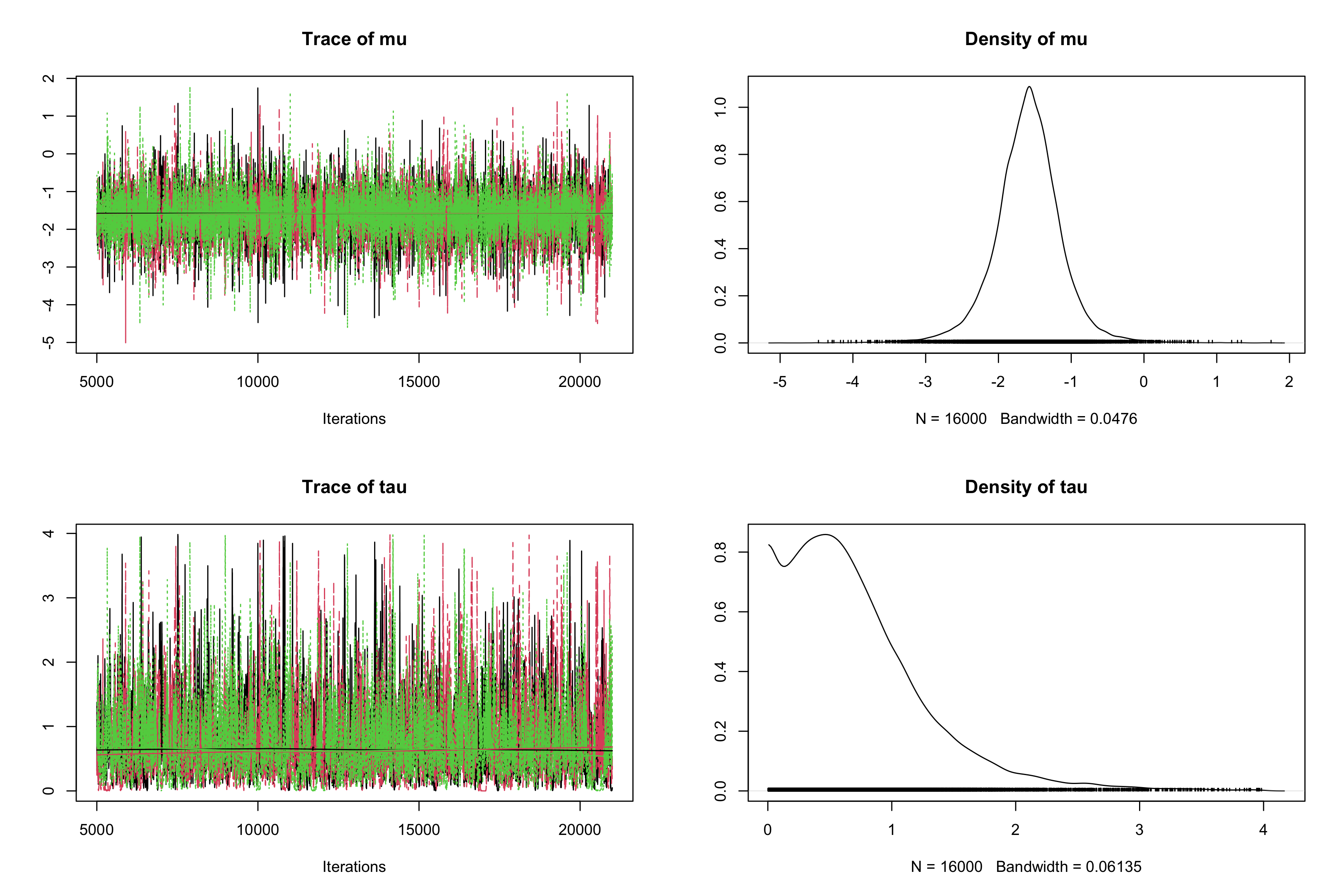

Nicola D Crins et al. “Interleukin-2 Receptor Antagonists for Pediatric Liver Transplant Recipients: A Systematic Review and Meta-Analysis of Controlled Studies,” Pediatric Transplantation 18, no. 8 (2014): 839–850, doi:10.1111/petr.12362.↩︎
Christian Röver “Bayesian Random-Effects Meta-Analysis Using the Bayesmeta R Package,” Journal of Statistical Software 93 (2020): 1–51, doi:10.18637/jss.v093.i06.↩︎
Joseph L. Fleiss and Jesse A. Berlin “Effect Sizes for Dichotomous Data,” in The Handbook of Research Synthesis and Meta-Analysis, 2nd Ed (New York, NY, US: Russell Sage Foundation, 2009), 237–253.↩︎

Last updated on June 18, 2025

Edit this page